

The dedicated measurement and interpretation of solar oscillations evolved into a new field called helioseismology , mainly developed in the last fifty-four years, but few lay folk are aware of it.. However, plumbing the Sun's depths to investigate its different modes of vibration allows hitherto unknown tools to be applied to many types of solar predictions.
Helioseismology began more or less formally in the 1960s when Robert Leighton and colleagues discovered oscillations on the surface of the Sun. Leighton was actually looking at specific wavelengths associated with solar granulation. e.g.

And expected as the images got further apart in time they'd exhibit less coherence. But instead he found that after 5 minutes they were back in phase, i.e. reinforced. This marked the discovery of the 5 minute oscillations.
A few years later John Leibacher and associates theorized the origin as acoustic waves trapped in a cavity just below the solar surface. These were generated by blobs of hot gas at the top of the Sun's convective zone. This led to the first reckoning of non-radial oscillations ca. 1968 with two-dimensional plots of wavenumber vs. frequency or (k -w) diagrams. In typical k -w diagrams, we have frequency w along the ordinate and k along the abscissa. One would then see the p-modes in the upper left lying above w ac and the g-modes (gravity modes) at lower right below a dotted line for N. Another line given is for ckh which represents the Lamb waves or f-modes.
Several peaks of amplitude were found and it was suggested that these corresponded to the fundamental and first overtones for the solar envelope. Interestingly the patterns of solar oscillations - namely the acoustic or "p-modes" resemble those detected on drum heads by computer holography. The regions for p and g modes are depicted in the artist's diagram below:
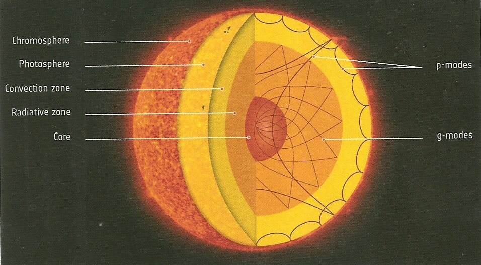
The Sun is clearly not a drum head, but it seems to behave like one in terms of its oscillations. Solar physicists are particularly interested in what are called p, g and f modes given they are resonant modes of oscillation. The p-modes are basically associated with acoustic or sound waves, the g modes are for internal gravity waves and the f modes are for surface gravity waves.
The waves as noted above, have been found to have a roughly 5-minute period, and solar physicists have discovered about 10 million modes for the waves - with roughly one million of these shaking the surface at any one time. A computer- generated image of some of the waves is shown at the top of this post. How is 10 million arrived at? This has to do with the spherical harmonic mathematics which we will get to. For now, we note the key function for all distinct (n, ℓ and m) p-modes, is specified by y nℓm
Let’s take n first. According to diagnostic diagrams showing
“ridges” for oscillatory power at each frequency, e.g.

at least 20 have been observed. In the diagram shown, the spikes or ridges for the p-mode represent the first harmonic and the baseline smooth curve from which they project is the fundamental. This leads to a maximum radial order of n = 20 for the p-mode associated ridges.. Now, for each of these n values, at least 500 angular degrees ℓ have been observed. We also know that for each such ℓ there are at least 2 ℓ values (actually 2 ℓ + 1). So in this case:
2 ℓ = 2(500) = 1000.
Then the total estimated modes at any given time works out to:
T
n ℓm
= 20 x 500 x 1000 = 10 7
Or, ten million modes, all overlapping in time and space
Like the seismic waves that affect Earth, often before earthquakes, the Sun's waves have important diagnostic capabilities. We know, for example, that as the waves travel into the Sun they're refracted toward the surface by changes in temperature, density and composition. Individual waves, then, are re-directed differently depending on the foregoing properties at the given location, as well as the path of propagation through the Sun. A careful analysis of the waves thereby provides a detailed look at conditions deep in the Sun. Helioseismology, in fact, is the only know way to see deep inside our star.
It has been Dopplergrams making use of the Michelson Doppler Imager (MDI) that have given us the best observation portal on the rising and falling super cells known as supergranules. In the Doppler image shown at the top the dominant motion is for solar rotation, so we see the eastern side of the disk is blue shifted, while the western side is red shifted. (Moving away from us). Waves at the surface create the fuzzy appearance of the disk overall.
The necessary wave analyses, of course, entail mathematical methods that make use of already well-known functions applicable to similar physical systems.
Enter the spherical harmonic function, which is also peculiar to atomic physics, but here is most applicable to the p-modes . In the solar oscillations context, the key function, as I noted, is given by:
y nℓm = R n (r) Y ℓm (q, j) exp (i w t)
Here, R n (r) is
applicable to radial patterns (with n the radial quantum number) whereby for a
given value of n we elicit a pattern of radial nodes, for which the position is
determined by the exact pattern of the function
R n (r) The rest of y gives the surface pattern as a spherical
harmonic of the oscillation. The spherical harmonic, e.g.
Y ℓm (q,j),
determines the angular (q,j) dependence of the eigenfunctions and hence the surface distribution of the oscillation amplitudes, i.e. as seen by an observer. The letters n, m and ℓ denote numbers whose meanings should be further clarified. The first is the radial order or the number of nodes in the radial direction. The second is the harmonic degree or azimuthal order which indicates the number of nodes around the equator on the three dimensional spherical surface.
Finally we have the angular degree or the number of nodes from pole to pole, e.g. along longitude or meridian lines. The difference (ℓ - m) is also of interest as it yields the lines corresponding to parallels of latitude. Any given combination of the numbers n, m and ℓ allows a unique frequency n to be computed. For example, if we have n= 14, m = 16 and ℓ = 20 one gets a period of 340.61 s or:
n = 2 p/ T = 2 p/ (340.61 s) = 2.935 x 10 -3 /s
Radial oscillations alone have ℓ = 0 and we see in this case the associated Legendre function P ℓm (q ) has:
P ℓm (q ) = (1 – z2) m/2 / ℓ! 2ℓ d (ℓ+m) / dz(ℓ+m) (z2 -1) ℓ
Recall m= 2 ℓ + 1 = 2(0) +1 = 1
So:
P ℓm (q ) = (1 – z2) 1/2 / 0! 20 d / dz (z2 -1) 0
= (1 – z2) ½ = (1 – cos 2 q)½ = (sin 2 q)½ = sin q
For q = p/2 , P ℓm (q ) = 1
And: P ℓm (q ) exp (i m j) = (1) exp (i (1) 0) = 1
If n nℓm = 1 c/s
then: Y ℓm (q,j) = 1 and y nℓm = R
n (r)
The degree ℓ of the spherical harmonic can assume any integer value, i.e.:
ℓ = 0, 1, 2, …….
At
each such ℓ the azimuthal number m assumes a 2 ℓ +
1 value, i.e.
m= - ℓ, (-ℓ +1)....0......( ℓ - 1), + ℓ
Meanwhile, the frequency of a particular mode is
given by the azimuthal eigenvalue m, and the meriodonal eigenfunction ℓ - together with n. Since m= 2 ℓ + 1, then the spherical
surface is split into 2 ℓ + 1 regions.
Hence,
there exist ℓ values of q for
which the function P ℓ (m )
vanishes. The zeros occur on specific parallels of latitude on the
sphere. All odd-numbered harmonics vanish at the equator given they contain the
factor m = cos q.
Hence at the equator q = 90
degrees so cos (90) = 0. In like manner, P m ℓ (m)
vanishes along (ℓ - m) parallels of latitude. The associated
functions vanish at the poles (m = +1) when m >
0. The zeros at the poles are of order m/2 because of the factor
:
(1
- m 2 ) m/2 in the
general equation.[1]
The first few zonal harmonics are computed using an alternative form of Rodrigues’ formula,
P ℓ (m) = 1/ (2 l ℓ!) d 2 / d m 2 ( m 2 - 1) l
Then: P 0 = 1
P 1 = m
P 2 =
3 m 2
/2 - ½
This, alas, is about as far as we can go without getting "too much in the weeds." Let me just end this post by noting that in 1981, Leibacher and Stein showed that if one treated the Sun as a resonant cavity one could expect the relationship between period, T and frequency, w :
T
= (n + ½)p / w
In other words for the condition at which the sound speed equals the horizontal phase velocity (w/k h ) one expects acoustic wave reflection. Duvall and Harvey [2] reinforced this work by measuring the frequency spectrum of this » 300s oscillation and found it applicable for ℓ-modes less than 140, and radial modes R with order n = 2 to 26. Posing the degree ℓ- in terms of the reflection radius r:
ℓ =
-1/2 + [ ¼ +
4p2 g2 r2 / c2 ]
The
modes were thus established as being deep in the solar interior by matching all
the modes in a series of data using the above equation.
----------------------
-----------------------------
Suggested Challenge Problem:
Explain the appearance of the spherical surface shown below if it describes m= 5 and ℓ = 5. Thence, find the associated Legendre function: P ℓm (q ) and also Y ℓm (q,j) assuming q = p/2: (Assume n nℓm = 1 /s)

No comments:
Post a Comment