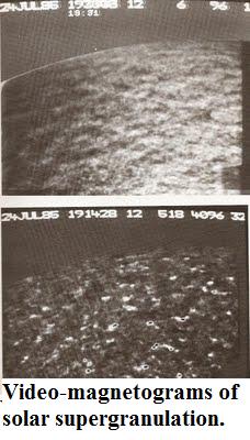
We continue now examining Jason Lisle's primary claim to fame, as embodied in his Ph.D. thesis and some papers spun off from it, concerning finding a "persistent N-S alignment" for solar supergranules, taken to be a polarity preference associated with their directions.
Very early in his dissertation (p. 17), Lisle concedes an inability to properly resolve granules via his Michelson Doppler Imager (MDI) velocity data, though he does make an appeal to local correlation tracking (LCT) as a kind of savior since it allows motions to be deduced from the images even when individual moving elements aren't well resolved. (I.e. the granules are the individual elements or units of supergranules). The question that arises, of course, is whether this product of such LCT manipulation is real, or to put it another way, an objective physical feature that is not associated with instrumental effects, distortions or errors.
Exacerbating this suspicion is Lisle's own admission (ibid.) that LCT "suffers from a number of artifacts". Indeed. Any central heliographic artifact which sports velocity motions of magnitude 200 m/s - and hence overpowers (by a factor TEN) that signal which one is seeking, is bound to cause havoc and efforts at resolving the signal are likely to be dubious at best...if the right instruments or reduction methods aren't employed. Does Lisle employ them?
He thinks he does, but I beg to differ. At least to his credit he admits (p. 21, Thesis) the enormous mismatch between the magnitude of his sought signal and his unwanted artifact noise. He also concedes the artifact is a selection effect and a product of his very LCT algorithm! (The algorithm preferentially selects the central blue-shifted cores of any granules moving toward the heliographic center, and hence exaggerates the associated velocities.) Fair enough. So what's the solution for removing them?
He claims to be able to "reproduce" the disk-centered false flows and also (presumably by doing this) "account for' many of their properties. But this is disputable, especially given he chooses to replace the velocity component of his LCT flow field with Doppler velocity data. While plausible sounding in theory, in practice it's a different matter, as we learned at the 40th meeting of the Solar Physics Division in Boulder, in 2009. The reason? "Dopplergrams" often betray false motions, by virtue of exhibit brightness variations in different (spectral) bands which may not always arise from motions! Thus, differential brightness changes observed in dopplergrams may yield motions that are erroneous. This means they can't be used as consistently reliable indices for velocity especially anywhere near the solar photosphere. (At the particular session devoted to dopplergrams it was pointed out that we need to use maps of subsurface flows in conjunction to obtain accurate readings).
My point here is that if he indeed substituted Dopplergrams to get his velocity component, then he in effect inadvertently added another systematic error on top of his selection errors associated with the large scale flow artifact.
More worrisome are the admissions in the paper he co-authored with Toomre and Rast (Astrophysical Journal paper (Vol. 608, p. 1170), 'Persistent North-South Alignment of the Supergranulation'):
supergranular locations have a tendency to align along columns parallel to the solar rotation axis.... this alignment is more apparent in some data cubes than others… The alignment is not clearly seen in any single divergence image from the time series of this region (Figs. 1a–1b) but can be detected when all 192 images comprising that series are averaged”
But why should these alignments be more evident in some data cubes than others? Lisle's "solution" is to devise "merit tiles" or tiny sub-sections of data- roughly of meso-granule size (i.e. midway between granule and super-granule) that encompasses the grid points he's selected. He then renders all these merit tiles uniform and with dimensions 5 pixel x 5 pixel, where each pixel scale is ~ 2 arcsec in full disk mode. He asserts this corresponds to 1.4 Mm at the solar center, and "comparable" to the size of a typical supergranule, or 1.0 Mm. However, there is in fact a 40% difference in scale, and what the Dopplergrams velocity profiles will do is increase it.
His next ploy is to resort to "shifting" these tiles by "sub-pixel" amounts in latitude (y) and longitude (x) directions, whereby any tile shifted by delta(x) and delta (y) is compared to the corresponding tile at the same grid point in the in the subsequent image in time. He then claims to be able to evaluate a "correspondence" between any such two tiles according to a "merit function": m(delta(x), delta(y)).
This again is suspect, because if he's using velocity components from Dopplergrams, with their systematic errors (which he doesn't say were ever accounted for) there's no assurance that subsequent tiles will really show the same grid points, far less at the same time (since a systematic delta(v) will shift them). Thus, his "Gaussian weighting function" W, which he then applies to his merit functions (already clearly macguffins) isn't much use.
Going back to the same Ap.J. paper of Lisle et al, the authors write:
“After 8 days of averaging, the striping is quite strong, while shorter averaging times show the effect less well. In Figure 3a, s[x], s[y] , and their ratio s[x]/s[y] are plotted as a function of averaging time. The plots show the average value obtained from two independent well-striped 15 deg x 15 deg equatorial subregions of the data set”
In the above, s[x], s{y] refer to the rms or root mean square errors applied to the merit function components delta(x) and delta(y). Note also that longer averaging times correspond to more efficient noise, or unwanted signal, removal! (And as we know averaging or time averages in general, eliminate many aberrant signals - just like long term stock averages minimize and ground out large dips!) This is what we'd expect too from inclusion of any systematic errors in the v-component of granules associated with the use of Dopplergrams, i.e. the shorter the averaging times (or evening out) the less evident the wanted signal.
We're also alerted in the same paper to the asymmetrical rms errors for s[x] and s[y]:
s[x]/s[y] shows a smooth transition from values near one at low averaging times to values exceeding 2.5 for the full time series. This increase reflects the slow decrease in x compared to y due to the underlying longitudinal alignment of the evolving flow. The random contributions of individual supergranules to s[x] or s[y] scale as 1/(Nl)^½, where Nl is the number of supergranular lifetimes spanned over the averaging period.
Of course, being unaware of the influence of the anomalous v-component introduced by Dopplergrams this is a natural conclusion to make, that is, that a preferential persistence is displayed in x as opposed to y. However, if the Dopplergrams have introduced systematic errors in v as I am convinced, it is more plausible that we are seeing the emergence of asymmetric ERRORS in s[x] over s[y]. (Such that s[x] ~ 2.5 s[y]].
The confirmation of this spurious effect for me is when the authors write:
Vertical striping of the average image emerges visually when the averaging time exceeds the supergranular lifetime by an amount sufficient to ensure that the contribution of the individual supergranules falls below that of the long-lived organized pattern.
In other words, to control the signal to obtain the effect they need they have to resort to time averages t(SG) < T(P), where T(P) denotes the lifetime of the organized pattern.
How would they have fared better, and uncovered the likely systematic error in v from the Dopplergrams? They ought to have applied the statistical methods described by James G. Booth and James P. Hobert ('Standard Errors of Prediction in Generalized Linear Mixed Models', appearing in The Journal of the American Statistical Association (Vol. 93, No. 441, March 1998, p. 262) in which it is noted that standard errors of prediction including use of rms errors, and ratios thereof are "clearly inappropriate in parametric models for non-normal responses". This certainly appears to apply to Lisle et al's polarity "model" given the presence of significant "false flows" and "large convergence artifacts" (the latter with 10 times the scale size of the sought signal).
Booth and Hobert, meanwhile, recommend instead a conditional mean-squared error of prediction which they then describe at great length. They assert that their methods allows for a "positive correction that accounts for the sampling variability of parameter estimates". In Lisle et al's case, the parameters would include the propagation speed of supergranule alignments, after their s[x]/s[y] is replaced by the rubric offered by the J. Am. Stat. Soc. authors, including the computation of statistical moments (p. 266) to account for all anisotropies and other anomalies which appear. (The v-component anomalies ought to emerge in the statistical moments, most likely the 2nd).
Until this is done, it cannot be said that there exists any "persistent alignment" in the solar supergranulation! Fortunately for Lisle, at least his Thesis and subsequent papers do convey the pretense of actually knowing something - as opposed to the insipid bollocks of his "Young Sun" gibberish - which would be an embarrasment to any real astrophysicist - in terms of taking ownership for. (If his inveterate defenders to the effect Lisle's a "real astrophysicist" really had a grain of sense -which I doubt- they'd convince him to drop his 'Young Sun' crap forthwith, which makes a mockery of the claim of ever being able to write a Ph.D. thesis on his own. It just doesn't jibe!)
Let us also make clear one last thing for his noisome little cheerleaders who insist on crawling out of their trenches, caves and cubbyholes from time to time: anytime one talks about "biblically based" and scientifically proven one is talking of classes of logic and analysis 180 degrees apart. In fact, "biblical based science" is the biggest oxymoron there is. An oxymoron for all MORONS!
No comments:
Post a Comment