But sadly, as the piece by Bob Berman observes, while "professional astronomers use math all the time" - see e.g. some of the (free) journal articles here:
http://iopscience.iop.org/0004-637X/743/2
Hobby astronomers generally "don't have math in their bones". As Berman adds:
"They hate the subject. Perhaps it reminds them of school. Square roots and standard deviations bog down articles for them, and science writers oblige by leaving out equations altogether."
Which is sad beyond measure, because indeed, as Berman goes on to show, math is the language of the universe. Sure it's easy to simply stand beneath the stars and simply gaze at galaxies, planets and the Moon through a telescope - Oooh-ing and ahh-ing all the time. But while wonder and awe can be the keynote at that level, it can't lead to any deeper understanding of what those objects actually are, what they're made of, how they move or how they might affect our planet. For that, deeper analysis is needed, i.e. into the relationships between physical parameters that define them.
Just to know how distant an object is - say a nearby star- depends on math, and it is critical given that the distance can allow other properties to be determined. Consider the famous "parallax method" to obtain the distance to nearby stars. This method can apply to all stars within a distance of maybe 50 parsecs (1 pc = 3.26 Ly) or those for which a measurable parallax angle p exists. The geometry shown below is useful to this end:

The angle p is obtained by taking photographs of the same star six months apart (i.e. from opposite sides of Earth's orbit) and comparing the two positions. One can thereby obtain the distance, D from:
D = r/ tan (p)
The relationship is such that for p = 1 arcsec the distance of the star would be 1 parsec (e.g. par-allax sec-ond). an angle of 1 arcsec = 1" = 1/3600 degree. So we see it is an extremely tiny angle. similarly, if the angle p = 1/10" then D = 10 parsecs, so we perceive a reciprocal relationship such that D = 1/p", though we must ensure the units are consistent.
In many applications, such as the budding undergrad student meets in 1st year Astronomy, the parallax angle p is merged with the equation for the "distance modulus" - which makes use of the absolute magnitude M (see previous blog on this) and apparent magnitude m. In this way, estimates of the star's energy output, and brightness can be made.
Then, if D is the distance, the usual expression for distance modulus is:
(m - M) = 5 log (D/10) = 5 log D - 5 log 10 = 5 log D - 5
But: D = 1/p
so:
(m - M) = 5 log (1/p) - 5
Or: (m - M) + 5 = 5 log p
A sample problem, such as an Astronomy 201-202 student would have to do for homework, is as follows:
Barnard's star has an absolute magnitude of +13.2 and an apparent magnitude m = +9.5. Find its distance in LIGHT YEARS.
The solution is based on using the parsec form of the distance modulus:
Then:
(m - M) = 5 log (1/p) - 5
(9.5 - 13.2) = 5 log(1/p) - 5
-3.7 = 5 log (1/p) - 5
5 log (1/p) = (5 - 3.7) = 1.3
log (1/p) = (1.3)/5 = 0.26
Taking anti-logs:
1/p = D = 1.81 pc
But 1 pc = 3.26 Ly, so D = (1.81 pc)(3.26 Ly/pc) = 5. 9 LY
Spherical Astronomy:
We are looking at how math drives our understanding of the universe from the perspective of a budding astronomy major at university. By the time the aspiring major reaches his sophomore year, he will be facing even more math in courses such as Spherical Astronomy. The emphasis here is on astronomical time (sidereal time and position - the latter based on different coordinate systems used (equatorial, horizontal, ecliptic). Each such coordinate system is defined by a different set of poles and equator. For example, the coordinate system depicted in the diagram below is known as the equatorial system.

It is based on the projection of the Earth's N. and S. poles into the sky, as well as its equator. The poles then become the North and South Celestial poles, and the equator becomes the celestial equator. If these poles are defined respectively at +90 degrees (NCP) and -90 degrees (SCP) and the celestial equator at 0 degrees, then a consistent system of celestial latitude and longitude can be defined in a consistent system, to locate any celestial object. We call the longitude coordinate (Θ) the Right Ascension (R.A.) while the celestial latitude coordinate is called declination and is measured in degrees north or south of the celestial equator. (In the diagram, the complementary angle of the declination is shown, φ, which we call the zenith distance.)
One of the first things the astronomy sophomore learns is how to find directions around the celestial sphere, including how to relate the R.A. to time and time keeping. He must also do exercises showing he can find the hour angle - and distinguish it from the Right Ascension. This starts with identifying the R.A. of his local meridian (the imaginary celestial longitude passing through his zenith or highest point.) The Right Ascension of the star is clearly equal to the local sidereal time (L.S.T.) plus the hour angle. Thus, we can write: HA = RA of observer meridian - RA of object
Of course, before he gets very far, he will be adept at sketching any number of diagrams to solve time and position problems, such as the diagram below - with perspective looking down onto the North Celestial pole:

For example, in the diagram shown, if the star's R.A. is 7h 00m and the observer is at a local sidereal time of 6h 00m, then the hour angle becomes: HA = 6h - 7h = -1h or -15 degrees. (Since every hour of longitude corresponds to 15 degrees angle, i.e. Earth turns through 15 degrees every hour, 360 degrees in 24 hours.)
The budding astronomy student will also have to know how to sketch a three dimensional diagram to enable conversion between coordinates, say from the horizontal (observer -based) to the celestial sphere. This will always include what is called the fundamental "astronomical triangle" (shaded region of Fig. 3 below):
The budding astronomy student will also have to know how to sketch a three dimensional diagram to enable conversion between coordinates, say from the horizontal (observer -based) to the celestial sphere. This will always include what is called the fundamental "astronomical triangle" (shaded region of Fig. 3 below):
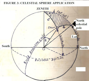
from which spherical trig relationships can be obtained and conversions can be made to different coordinate systems. Using spherical trig, the student can write the law of sines and law of cosines for spherical triangles (such as shown in Fig. 3)which are analogs of the law of sines and cosines for triangles in plane trig.
We have for the law of sines:
Sin A/ sin a = sin B/ sin b = sin C/ sin c
where A, B, C denote ANGLES and a,b,c denote measured arcs. (Note: we could also have written these by flipping the numerators and denominators).
We have for the law of cosines:
cos a = cos b cos c + sin b sin c cos A
Where a, b, c have the same meanings, and of course, we could write the same relationship out for any included angle.
Now, we use Fig. 3, for a celestial sphere application, in which we use the spherical trig relations to obtain an astronomical measurement.
Using the angles shown in Fig. 3 each of the angles for the law of cosines (given above) can be found. They are as follows:
cos a = cos (90 deg - decl.)
where decl. = declination
cos b = cos (90 deg - Lat)
where 'Lat' denotes the latitude. (Recall from Fig. 1 if φ is polar distance (which can also be zenith distance) then φ = (90 - Lat))
cos c = cos z
where z here is the zenith distance.
sin b = sin (90 deg - Lat)
sin c = sin z
and finally,
cos A = cos A
where A is azimuth.
Let's say we want to find the declination of the star if the observer's latitude is 45 degrees N, and the azimuth of the star is measured to be 60 degrees, with its zenith distance z = 30 degrees. Then one would solve for cos a:
cos a = cos (90 deg - decl.)=
cos (90 deg - Lat) cos z + sin (90 deg - Lat) sin z cos (A)
cos (90 deg - decl.) =
cos (90 - 45) cos 30 + sin (90 - 45) sin 30 cos 60
And:
cos (90 deg - decl.)= cos (45) cos 30 + sin (45) sin 30 cos 60
We know, or can use tables or calculator to find:
cos 45 = Ö2/ 2
cos (90 deg - decl.)= cos (45) cos 30 + sin (45) sin 30 cos 60
We know, or can use tables or calculator to find:
cos 45 = Ö2/ 2
cos 30 = Ö3 / 2
sin 45 = Ö2 / 2
sin 30 = ½
cos 60 = ½
Then:
cos (90 deg - decl.) = {Ö2/ 2)(Ö3 / 2)} + {Ö2/ 2} (½) (½)
cos (90 deg - decl.)= [Ö6/ 4 + Ö2/ 8]
= {2Ö6 + Ö2}/ 8
cos (90 deg - decl.)= 0.789
arc cos (90 deg - decl.)= 37.9 deg
Then:
decl. = 90 deg - 37.9 deg = 52.1 deg
Or, decl. (star) = + 52.1 degrees
The student will also become familiar with matrix methods for converting between the different coordinate systems.
The basic principle involves relating the Cartesian coordinates (rectilinear) of a point on the celestial sphere (diagram) to the curvilinear coordinates measured in the primary and secondary reference planes. One has then, for example:
(x)
(y)
(z) u,v =
(cos v .....cos u)
(cos v .....sin u)
(sin v..............)
After conversion the curvilinear coordinates may be calculated according to:
(x)
(y)
(z) u,v =
(cos v .....cos u)
(cos v .....sin u)
(sin v..............)
After conversion the curvilinear coordinates may be calculated according to:
u = arctan (y/x) and v = arcsin (z)
Now, consider conventional orthogonal matrices of 3 x 3 dimensions, given as functions: R1(Θ), R2(Θ) and R3(Θ), to rotate the general system by the angle Θ about axes x, y and z, respectively. Thus we obtain:
R1(Θ) =
(1..........0................0)
(0.....cos(Θ)..... sin(Θ))
(0......-sin(Θ)....cos(Θ))
R2(Θ) =
(cos (Θ)......0........- sin(Θ))
(0................1...............0.. )
(sin(Θ)........0.......cos(Θ) )
R3(Θ) =
(cos(Θ)..........sin(Θ)..........0)
(-sin (Θ)......cos(Θ)...........0)
(0 ..................0..................1)
To fix ideas, say you wish to obtain the horizontal coordinates (A, a) for some object in the sky and you know its R.A. and decl. from an almanac. Then the procedure is fairly straightforward, and entails writing:
R3(Θ) = R3(-180 deg)
R2(Θ) = R2(90 - lat.)
so that:
(x)
(y)
(z) A,a = R3(-180 deg) R2(90 - lat.) (XYZ(h, decl.))
R2(Θ) = R2(90 - lat.)
so that:
(x)
(y)
(z) A,a = R3(-180 deg) R2(90 - lat.) (XYZ(h, decl.))
where : (XYZ(h, decl.)) =
(x)
(y)
(z) h,decl.
(x)
(y)
(z) h,decl.
Bear in mind: R3(-180 deg) =
(cos 180........-sin 180................0)
(sin 180........cos 180................0)
(0......................0......................1)
(cos 180........-sin 180................0)
(sin 180........cos 180................0)
(0......................0......................1)
And:R3(Θ) =
(cos(Θ)..........sin(Θ)..........0)
(-sin (Θ)......cos(Θ)...........0)
(0 ..................0..................1)
Therefore: R3(-180) =
(-1.....0.......0)
(0.......-1.....0)
(0.......0.......1)
Obtaining R2(Θ) = R2(90 - lat.) is just as easy, if one recalls the basic trig identity:
cos (90 - φ) = sin (φ)
Not surprisingly, it is the sophomore year at which point most wannabe Astronomy majors change their minds and either drop out entirely or change their major - say to a less mathematically demanding subject. At the Univ. of South Florida, nearly 60% had dropped out by the end of the quarter which featured spherical astronomy.
Astrophysics:
In Introductory Astrophysics, the primary emphasis is getting the student acquainted with the Planck function and applying it to simple, plane-parallel stellar atmospheres, such as depicted below:

The Planck function describes the distribution of radiation for a black body, and can be expressed:
B(l) = {(2 hc2)/ l5} [1/ exp (hc/lkT) - 1)]
Of course, all stars are effectively black bodies, which are perfect radiators, or as close to that state as nature allows. In the case of simple radiation transfer in a static model stellar atmosphere (e.g. nothing changes with time), we have the relation of specific radiation intensity I(l) to source function S(l):
dI(l)/ds = -k(l) I(l) + k(l) S(l)
= k(l) [S(l) – I(l)] - 0 or I(l) = S(l)
For a black body, the student learns I(l) equals the Planck function:
B(l) : i.e. S(l) = I(l) = B(l)
And this is a condition which implies LOCAL THERMODYNAMIC EQUILIBRIUM or LTE LTE does NOT mean complete thermodynamic equilibrium!(E.g. since in the outer layers of a star there is always large energy loss from the stellar surface) . Thus, one only assumes the emission of the radiation is the same as for a gas in thermodynamic equilibrium at a temperature (T) corresponding to the temperature of the layer under consideration. Another way to say this is that if LTE holds, the photons always emerge at all wavelengths. In the above treatment, note that the absorption coefficient was always written as: k(l) to emphasize its wavelength (l) dependence.
The student will be required to do a number of challenging problems for homework, including the specific applications of the gray atmosphere approximation. In a particular integral, let the surface flux:
p( Fo ) = 2 p (I(cos (q)) = p [a(l) + 2(b(l)/3 ]
and Flo = S(l) t(l) = 2/3
which states that the flux coming out of the stellar surface is equal to the source function at the optical depth t = 2/3. This is the very important ‘Eddington-Barbier’ relation that facilitates an understanding of how stellar spectra are formed. Once one then assumes LTE, one can further assume k(l) is independent of l (gray atmosphere) so that:
k(l) = k; t (l) = t and Flo = Bl (T(t = 2/3) )
Thus, the energy distribution of Fl is that of a black body corresponding to the temperature at an optical depth t = 2/3. From this, along with some simple substitutions and integrations a wdie array of problems can be done. A few HW problem examples:
1. Estimate the specific intensity I (q=p/4) if the surface flux from the Sun is 6.3 x 10 7 Jm-2 s-1.
2. Find the effective temperature of the Sun and the boundary temperature (To) and account for any difference. (Hint: The effective temperature is related to the boundary temperature by: Teff = (2)1/4 To )
At some later stage sources' radiation characteristics will also be covered, and this will include treating the quantity known as the specific intensity i.e.
Il (0,q) = òo z Bl(t) exp [(-tl / cos q)] dt/ cos q
where Bl(t) is the Planck function. The energy which flows per unit solid angle will then be based upon finding:
dE n = I cos q dw dt dn
from which one will wish to obtain the total flux.
By now radio astronomy will emerge, with essentials of assorted radio telescope properties, especially for antennas, will also be introduced, along with many problems - including practical (i.e. designing a specific antenna to detect an object of given flux, and spectral output etc.). To this end the student will distinguish between the flux emitted for an isotropic (lossless) antenna, and an anisotropic antenna with the gain (g) subject to the constraint:
ò 4p g dw = 4p
and the relation between the gain of the antenna and its effective aperture (A) such that:
g( (q , φ ) = 4p A (q , φ)/ l2
From here, the student will be expected to work out the beam width and beam efficiency of a given antenna, as well as compute the 'brightness temperature' for a localized source, and the antenna temperature:
Ta = 1/4p ò 4p g T(b) dw
where T(b) is the brightness temperature.
Sensitivity of the antenna will also be considered, as well as other details such as the amplification of high frequency signals.
Sensitivity of the antenna will also be considered, as well as other details such as the amplification of high frequency signals.
By his senior year, the budding astronomy major will have to confront the theory of stellar structure. In this case, the student will be introduced to a variety of differential equations which he'll later be expected to use in the construction of an actual stellar model (which may be 50 percent of his final grade.) He learns that the force of attraction between M(r) e.g. the mass enclosed inside the stellar sphere of radius, r and r dr (the mass of an element) is the same as that between a mass M(r) at the center and r dr at r. By Newton’s law this attractive force is given by:
F = G M(r) r dr/ r2
Since the attraction due to the material outside r is zero, we should have for equilibrium: - dP = G M(r) r dr/ r2
Or: dP/dr = - G M(r) r / r2
Consider now the mass of the shell between an outer layer of a given star and a deeper stellar layer. This is approximately, 4p r2 r dr, provided that dr (shell thickness) is small. The mass of the layer is the difference between M(r + dr) and M(r) which for a thin shell is:
M(r + dr) - M(r) = (dM/ dr) dr
Equating the two expressions for the mass of the spherical shell we obtain:
dM/dr = 4p r2 r
The two equations, for dP/dr and dM/dr represent the basic equations of stellar structure, without which the innards of a star would be inaccessible to investigation. A third equation of stellar structure may be derived using by using the equation for dM/dr in combination with the fact that a star’s luminosity is produced through the consumption of its own mass. This may be expressed mathematically as:
dL/dM = e
where e denotes the rate of energy generation. For the proton-proton cycle (for stars like the Sun- and designed for cgs units!):
e= 2.5 x 10⁶ (r X2).· (106 /T)2/3 exp[-33.8(106 /T)1/3]
Of course, to construct a stellar model as part of a course project, the student will more likely have to deal with a different 'critter' entirely - say a star of two solar masses with a convective (as opposed to a radiative) core and with composition: X = 0.65 (i.e. 65% hydrogen), Y = 0.32 (i.e. 32% helium) and Z = 0.03 (i.e. 3 % heavy elements). Say with an energy generation function:
e= 10-14.2 (r X X(CN)).· (T20 )
where: X(CN) = 0.01 and :
X = 4.34 x 1025 Z(1 + X) r T --3.5
This is none other than the stellar model problem construction I had to complete, and for which I received an 'A' and also an A in the course. The details of the problem were:
Neglect radiation pressure and degeneracy and assume the gas is nearly totally ionized. Utilizing Wrubel's interior integrations and Schwarzschild's and Harm's envelop solutions:
a) Construct a consistent stellar model utilizing the U-V plane fitting technique, and
b) Calculate the following physical properties of the star: L, R, Tc , r c , Pc , and the mass of the convective core, m c .
Still want to become an Astronomy major? Just make sure math is in your blood.
(This was published in 3 parts originally under the title 'Math Drives The Universe', in November, 2013)
No comments:
Post a Comment