One reason for a major split between the space physics and solar physics communities has been the efforts of the former discipline to account for solar flares without resort to changing magnetic configurations, or magnetic morphology. What they've tried to do then, is to impose auroral substorm structures (V-potential, S-potential) , parameters (magnetostatic Ñ · A = 0 inputs) and models on solar conditions to explain energetic events like flares. Many of these attempts have employed models that are based on dynamo analogs for magnetic substorms in the Earth's magnetosphere. The models are then teased into quantitative shape to try to show how they might explain solar flares, or even the much more fundamental magnetic shear in the photosphere.
I had my first encounter with these efforts while delivering a lecture (on magnetic complexity of active regions in relation to solar flares) at the Geophysical Institute in Fairbanks, AK in October, 1985, e.g.
This was in conjunction with the GI's ongoing seminar series to do with space physics, solar physics and geophysics topics. Halfway through my presentation - which included actual slides showing progressive magnetic shear (in vector magnetograms) and the visual effects of such in an active region, distorting the neutral line e.g.
And which can be seen in successive magnetogram images, e.g.
Progressive magnetic shear over Nov. 5-7, 1980 in AR 2776.
Attendee S.I. Akasofu (known for his modeling of auroral substorms) queried the physical significance of the shear and why an auroral approach would not be better. I replied that the physical conditions - as well as visible signatures - did not merit such an approach. I pointed out the image - among others- and that contour maps of such regions at discrete radio wavelengths disclosed the controlling influence of magnetic fields. Indeed, penumbral filaments of sunspots themselves occurred in vertical planes defined by the horizontal component of the magnetic field. None of this satisfied Prof. Akasofu who then blurted:
"See, all you solar physicists talk about magnetic shear but you have no idea what it really is!"
To which I replied:
"In fact we do know what it is, because we can actually detect it and see it in our H-alpha images and magnetographs. The very distortion of the magnetic neutral line in active regions proves this shear is real and can be quantified."
Akasofu in 1985 at the Geophysical Institute
Truth be told I was puzzled by Akasofu's intensity of objection and acrimonious response to solar physicists and the accepted concept of magnetic shear. It seemed disproportionate to the topic at hand, as if he had some 'skin' in the game that had to be defended. Only later, two years later, did I realize this was so on uncovering a paper he had produced with Joseph Kan and L.C. Lee - also based at the Geophysical Institute and Univ. of Alaska-Fairbanks.
This concerned their "Dynamo Flare" model (Solar Physics, Vol. 84, p.153, 1983) and how they sought to use it to account for flares. To be fair, their model commendably incorporated both energy generation and dissipation in one system, an aspiration long sought by multiple researchers to try to assay the energy output and balance. However, the model exhibited a number of defects which translated into a hidden “cost” for using such unobserved structures.
In general, their model overtaxed the similarity between substorms and solar flares, while ignoring key facts concerning the magnetic aspect of flares – such as the well-established relationship between magnetic complexity and important flares (e.g. Tanaka and Nakagawa.: Solar Physics, Vol. 33, p. 187, 1973)
Specific issues:
1) In their Dynamo model the “neutral wind” acts perpendicularly to the field –aligned ( J ‖ ) and cross-field (J ⊥ ) current. See e.g. their model structure in their paper from Solar Physics (1983) below:
Here the wind as described in their paper as a “shear flow” (p. 154) . The problem is that there is no evidence of such “neutral gas” in the region of the solar chromosphere or photosphere, nor of any consistent “flow” of the order of 1 km/s. Thus, it is an entirely fabricated construct bearing no similarity to real solar conditions. (Of course, adopting the positivist stance the authors can argue like Hawking does in his quantum coherence theory, that there is no correspondence to physical reality anyway, and it is only used to make predictions.)
More accurately, in the regions wherein real magnetic loops reside, the physical features of sunspots and their concentrated flux dominate. Thus, instead of some vague “neutral wind’ one will expect for example, a convective downdraft which helps to contain the individual flux tubes of a sunspot in one place (e.g. Parker, Astrophysical. J., 230, p. 905, No. 3, 1979.) The problem is that the downdraft velocity is not well-established and can vary from 0.3 to 1.5 km/s.(Parker, op. cit.)
In the proper space physics (magnetopheric) context, the “neutral wind” arises from a force associated with the neutral air of the Earth’s atmosphere (e.g. Hargreaves, The Solar-Terrestrial Environment, Cambridge Univ. Press, 1992, p. 24). This force can be expressed (ibid.):
F = mU f
where f is the collision frequency. It is also noted that this wind blows perpendicular to the geomagnetic field (ibid.)
If one solves for f above, and uses the magnitude of magnetic force (F = qvB) where B is the magnetic induction, and v the velocity one arrives at two horizontal flows for electrons and ions moving in opposite directions. mU f = qvB = (-e) vB = (e) vB
Thus,
v1 = mU f / (-e) B and v2 = mU f / (e) B
These ions and electrons thus move in opposite directions, at right angles to the neutral wind direction. Such “neutral wind” velocities are depicted in Kan et al’s Fig. 1 (into and out of the paper on the right side of their arch configuration) as ±Vn. In the magnetospheric system the current is always extremely small since the frequency is large. (Hargreaves, ibid). The region where the wind is most effective in producing a current in this way is known as “the dynamo region”.
Again, there is no similar quasi-neutrality in the solar case, since the ions and electrons move as one governed by the magnetic field in the frozen-in condition. This shows that the whole neutral wind concept has no validity in the solar magnetic environment.
2) In Akasofu, Kan and Lee's dynamo flare model, the dynamo action is required to send currents to specific regions to provide a Lorentz force: (J ⊥ X B). This implies a current system which is non-force free in contradiction to numerous existing observations, and the fact that at the level of the photosphere –chromosphere, the plasma beta:
b = r v2 m/ B2
is much less than 1. For example, contrary to their claim that the currents in the chromosphere are not parallel to the magnetic field, we have actual vector magnetographs which show otherwise. Further, we know gyro-resonance emission depends on the absolute value of the magnetic field in the region above sunspots, and contour maps of such regions at discrete radio wavelengths disclose the controlling influence of magnetic fields. Penumbral filaments of sunspots themselves lie in vertical planes defined by the horizontal component of the magnetic field. Again, both coronal and chromospheric gas pressures are insignificant relative to magnetic pressures, so fields in these regions must be at least very nearly force-free.
3) In the case of filaments or prominences in the low corona or chromosphere, the plasma would again have a very high magnetic Reynolds number, Âm = L VA / h
Where L is a typical length scale for a given solar environment, VA is the Alfven velocity and h is the magnetic diffusivity
The conductivity of the plasma would therefore be ‘infinite’ so that even a minuscule induced voltage arising from, E = -v X B (e.g. due to very small relative motion v) would produce an infinite current j = s E. The only way one avoids this unrealistic situation is to require the plasma motion in the filament to follow magnetic field lines rather than cut across them.
Clearly, the error being made in this case and others is the overextension of space physics structures (e.g. as applicable to the aurora) to the solar physics – and specifically the solar flare context. To be more precise, one can visualize (in the case of the aurora) bundles of open field lines that map to the region inside the auroral oval. Many of these field lines can be traced back to the solar wind. The configuration is such that one is tempted to conceive of a mechanism that links certain mechanical or dynamic features to the production of cross currents, including Birkeland currents.
In detailed auroral models it can be shown that the "dynamo currents" in such a process flow earthward on the morning side of the magnetic pole and spaceward on the evening side. The circuit can be visualized completed by connecting the two flows across the polar ionosphere, from the morning side, to the evening side. This is exactly what Kan et al have done in arriving at their “dynamo solar flare” model. That is, taken a mechanism that might be justified in the case of the aurora – and transferred it to the solar flare situation.
The problem inheres in the fact that circuits on the Sun – given unidirectional current flows – need not be driven by any “dynamo action” – or be part of any dynamo. Further, one doesn’t require a dynamo to have a conservative energy system to account for solar flares. It is possible to use the conservation of magnetic helicity in a more general topological context to explain energy balance – especially for large, two-ribbon flares.
4) Lastly, the final result (eq. (34)) obtained by Kan et al on the basis of the Poynting theorem is not uniquely tied to a dynamo model of the type they present, but to any MHD generator model (cf. T. Hill, . Solar-Terrestrial Physics: Principles and Theoretical Foundations,, D.Reidel Publ. 1983, p. 261) Thus, the rate of change of electromagnetic energy density is equal to the energy source (-E ·J) minus the divergence of the Poynting vector:
S = E X H = (E X B)/ mo , where mo is the magnetic permeability.
Perhaps what the episode at the G.I. seminar in Fairbanks most shows is the inadvisability of allowing emotions to cloud judgments or arguments. In science we relentlessly preach the need for objectivity and not allowing emotions to rule, but then we tend to forget science is carried out by flesh and blood beings who are not always able to easily separate their passions from the models and hypotheses invoked in their published papers.
Interestingly, Akasofu's emotional and magical thinking - with predictable erroneous results - extends to climate change as well, see e.g.
https://skepticalscience.com//akasofu-LIA-recovery.htm
Excerpt:
|  Akasofu's Magical Thinking was Wrong
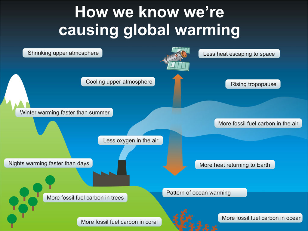
We know the increased greenhouse effect is creating a global energy imbalance that will cause the Earth's surface temperature to rise. Any alternative explanation has to identify why the increased greenhouse effect isn't causing the warming we expect based on fundamental physics, and why the climate change 'fingerprints' are consistent with the increased greenhouse effect. A brand new scientific journal called Climate published a paper by Syun-Ichi Akasofu, a retired geophysicist and former director of the International Arctic Research Center at the University of Alaska-Fairbanks. Despite having a background in physical sciences, Akasofu made a very unphysical argument in that paper. He claimed that the current global warming is merely a result of the planet “recovering” from the Little Ice Age – a cool period (the cooling mostly isolated in Europe) that lasted between the years of about 1550 and 1850. Problem – Akasofu didn’t identify any physical cause for this supposed ‘recovery.’ Instead he engaged in what’s known as “curve fitting,” in which you take data that is correlated to your desired graph and scale it to match, then argue you’ve proven that your data is the cause of the changes shown in that graph. In other words, it confuses correlation with causation. |


No comments:
Post a Comment