We now look at orthonormal bases.
The term sounds esoteric but many would have encountered it before either in
general physics or in advanced (AP) physics courses taken in high school. This
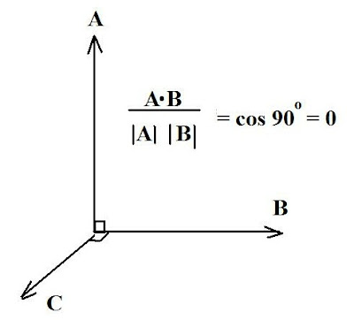
would be in conjunction with the dot product of vectors, such as illustrated in
Fig. 1.
Basically, in some Euclidean (straight line, 3D) system of coordinates, two vectors are considered orthogonal if their inner product is zero, as shown. The geometric properties here are assumed to be on the basis being orthonormal, i.e. composed of pairwise perpendicular vectors with unit length. Thus, in the figure shown, vectors A and B meet this condition (and the computation is shown for the vectors A, B) as do the vectors B and C. Then the vectors A, B, C meet the condition for an orthonormal basis.
Now, in applications of this concept, what the student is usually asked to do (say in his linear algebra course) is find an orthonormal basis for a "subspace" of R 3 (e.g. applied to a Cartesian space of three dimensions) which is generated by specified sets of vectors.
Example Problem (1):
Find an orthonormal basis for the subspace of R 3 generated
by the vectors (1, 1, -1) and (1, 0 ,1).
Solution: We let A
= (1, 1, -1) and B = (1, 0, 1)
The orthonormal basis for A is just:
A/ ‖A ‖ = (1, 1, -1)/ {12 +
1 2 + (-1) 2 } = (1, 1,
-1)/ Ö 3
The orthonormal basis for B is:
B/ ‖B ‖ = (1, 0, 1)/ {1 + 0 +
(1)2 } =
(1, 0 , 1)/ Ö 2
Of course, the beauty of linear algebra is that it can be generalized to
Euclidean spaces beyond the mundane 3, hence we can look at subspaces in R 4, generated by sets
of vectors (v1, v 2, v 3, v 4).
Example
Problem (2) :
Find an orthonormal basis for the
subspace of R 4 , generated by the vectors:
A = (1, 2, 1, 0) and B = (1, 2, 3, 1)
Solution:
For
A we have the orthonormal basis:
A/ ‖A ‖ = (1, 2, 1, 0)/ Ö{1 2
+ 2 2 + 1 2
+ 0 2 } =
(1, 2, 1, 0)/ Ö 6
For B we have:
B/ ‖A‖ = (1, 2, 3, 1)/ Ö {1 2
+ 2 2 + 3 2 + 1 2} =
(1, 2, 3, 1)/ Ö 15
Matrices and Eigenvalues:
a)Matrix Operation Basics:
The simple operation of matrix multiplication
such that, given a matrix A:
(a11 a12)
(a21 a22)
and a matrix B:
(b11 b12)
(b21 b22)
then A X B =
(a11 a12) (b11 b12)
(a21 a22) (b21 b22)
= [{(a11b11) + (a12b21)} --{(a11 b12)+ (a12 b22)} ]
[(a21b11) + (a22b21) } --{((a21 b12) + (a22 b22)}]
For example, let A=
(1 2)
(1 2)
and B =
(1 3)
(2 2)
then A x B =
(5 7)
(5 7)
The student should be able to work this out using the format shown. We now want
to extend this to further operations with matrices, and we will confine
attention to 2 x 2 matrices as subset of R 2.
Not all matrices multiply commutatively.
For example, with regular numbers it is a given that: (2 x
3) = (3 X 2) = 6
Thus, in symbolic form: a x b = b x a
and we say the multiplication is commutative. But this need not be so with
matrices and matrix multiplication.
For example, let: A =
(1 2)
(3 -1)
and B =
(2 0)
(1 1)
We find: A X B =
(4
2)
(5 -1)
But: B X A =
(2 4)
(4 1)
so that: A X B ≠ B X A
and matrix multiplication doesn't give the same result both ways.
Another application is to obtain the transpose of a matrix and repeat such
multiplication. The transpose of a matrix M, call it t^M, is obtained by the
following procedure:
Let M =
(m11......m12)
(m21.....m22)
Then t^M is obtained by switching
the elements such that for the
transposed matrix:
m11 = m11,
m12 = m21
m21 = m12 and : m22 = m22
Let A
=
(2...1)
(3...1)
Find: t^A:
Using the procedure shown above for
the elements, we have t^A =
(2.....3)
(1.....1)
Lastly, we come to the trace of a matrix. This is simply the addition of its
diagonal elements. Thus, for any matrix M such as denoted above:
Tr(M) = m11 + m22
The beauty of this is that it can easily be extended for any dimension matrix,
say 3 x 3, or 4 x 4 or whatever. You simply add the diagonal elements:
Find the trace of M1 =
(-1.....0.......0)
(0.......-1.....0)
(0.......0.......1)
We
easily see the diagonal elements and thence add them:
Tr(M1) = (-1) + (-1) + 1 = -2 + 1 = -1
Suggested Problems:
1) Recall t^A, found in Ex. 1
and let B =
(-1...1)
(1....0)
a) Find AB and thence: t^(AB)
b) Verify that: t^AB = t^B t^A
2) Find the trace of: R3(Θ) =
(cos(Θ)..........sin(Θ)..........0)
(-sin (Θ)......cos(Θ)...........0)
(0 ..................0..................1)
No comments:
Post a Comment