Statistical Mechanics Revisited (1)

Statistical mechanics (also statistical physics),  is that branch of physics  (according to Britannica.com) that combines the principles and procedures of statistics with the laws of both classical and quantum mechanics, particularly with respect to the field of thermodynamics.  This definition is useful for our purposes but also leaves out a lot, namely that what we have is a detailed probability theory (as mathematics oriented to physical states and spaces) applied to the behavior of microscopic particles.


The "Ising model" is central to many problems and systems in statistical mechanics.  It first came to the fore in the study of ferromagnetic systems. It was found that the use of such simplified models paved the way for greater understanding via modeling of more complex systems.  Let's now look at an elementary, statistical mechanical spin system.  A fairly  mundane example is a two-dimensional Ising model for ferromagnetic matter. It contains magnetic domains for which the individual spin magnets can be subject to sudden reversals. For a simple example, think of the 2D model of 4 x 4 elementary spin magnets as shown below:

 
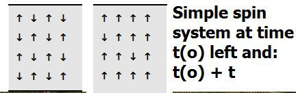
Here the Ising model system, by virtue of undergoing spontaneous magnetization  discloses an evolution to a higher degree of order  (from state S(1) to state S(2)) at the later time t(0) + t, where t could be in billions of years or nanoseconds.

The degree of order, as well as information, is determined from what is called "the spin excess", or the net spin difference (up minus down or vice versa). The larger this number, the greater the degree of order, and the lower the entropy of the system. Obviously, since 0 denotes an extremely low number, we can deduce large entropy.

Consider the system S(2) in more detail, noting the right side orientations of the elementary spin magnets. Here we get: 14 spin ups - 2 spin downs = 12 spin ups, or in other words the spin excess = 12. This system, S(2), has much higher degree of order (less entropy) than the system S(1). (We should add here that higher entropy - as in S(1) - corresponds to the most probable state, defined by the minimal spin excess of zero.)

Accessing such simple systems allows us to infer fundamental measures applicable to the systems, for example the "magnetic moment" of a state, as well as the "degeneracy function". Consider an N= 2 model system with either 2 ups (two up arrows) or 2 downs. 

Then, if  m  denotes the magnetic permeability we can have:

M = + 2 m   or M = -2 m

where the first is the magnetic moment for two spin- up particles, and the second for two spins down. One can also, of course, have the mixed state inclusive of one spin up plus one spin down, then:

M = O m or O

Meantime, the degeneracy function computes the number of states having the same value of m (individual spins) or M such that:

g(N,m) = N!/ (½N + m)! (½N - m)! [M_av]


where [M_av] denotes the average value of the total magnetic moment summed over all states (e.g. with m_s)

The power of the Ising model, however, doesn't end with ferromagnetic systems. We can also use it to examine ice crystal configurations as has been shown in a recent paper by Andrei Okounkov (Bulletin of the American Mathematical Society, Vol. 53, No. 2, p. 187).  In this paper the author presents us with the 2D ice crystal Ising model shown below:


Each white square denotes an ice crystal and the blue areas represent separating media. Certain model stipulations apply as given in the paper: 1) the total number of white squares is fixed, just as the total number of elementary magnets in the earlier system; 2) all squares along the boundary are deemed blue in order to prevent crystals sticking to the sides of the container, and 3) It must be possible to assign probabilities to the configuration in the same way we might assign "order" or entropy to the ferromagnetic system.

The most basic probability for any such system is "thermal equilibrium". Thus, at some temperature T if the system attains thermal equilibrium then the probability of any particular configuration decays exponentially with the energy of C, which is analogous to E  =  m _m  B in the ferromagnetic case. The probability of any particular configuration dependent on T is then:

Prob (C) = 1/ Z(T) [exp (-Energy (C)/ kT)

Where k is Boltzmann's constant, 1.38 x 10 ^-23  J /K.

One will also make use of the  "partition function":

Z(T) =  å _C   exp (- Energy (C)/ kT)

which as Okounkov notes, really functions as a "normalization factor"  given that it "makes the probabilities sum to 1".  In this Ising ice crystal model, then, the energy is "the sum of interactions of all adjacent squares." Since the total number of squares is fixed (see stipulation (1))  then the energy must be proportional to the total length of the contours separating white from blue.

To identify the contours is easy. If the energetic reader will run off  a copy of  the image of the 2D rectangle, then take a black magic marker and trace around each ice crystal region as it appears, he will have generated the contours. The normalization for energy is then (op. cit.):

Energy = 2 x Length of contours

As in the case of the ferromagnetic system entropy competes with order (energy).  In the Ising ice crystal energy is saved via clumping. If we designate an "order parameter" such that  b = (kT)^-1  then in the ice crystal case the larger   b   the stronger tendency for order. Interestingly, as Okounkov notes there is a critical temperature  T_c  > 0 above which entropy wins, it is:

b  =  0.5 ln ( Ö 2    + 1)  

Below T_c  and for ice crystal concentrations above a certain threshold a crystal will form as the size of the container goes to infinity.

Problems:

1) Quantify the magnetic energy for the system at time t(o) compared to time t(o) + t, if the magnetic energy of one spin magnet can be written:

M = - m B cos Θ

where m  is the magnetic moment (-eL/2m, L = 1) and assume Θ = +/- π, and B = 0.1T. 

2)  Say that S = log (g) determines the entropy for a  simple statistical mechanical system, where g denotes the number of accessible states. Then estimate S for the 2D ice crystal model - including any errors that might enter.