Statistical Mechanics Revisited (1)

Statistical mechanics (also statistical physics),  is that branch of physics  (according to Britannica.com) that combines the principles and procedures of statistics with the laws of both classical and quantum mechanics, particularly with respect to the field of thermodynamics.  This definition is useful for our purposes but also leaves out a lot, namely that what we have is a detailed probability theory (as mathematics oriented to physical states and spaces) applied to the behavior of microscopic particles.


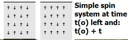
The "Ising model" is central to many problems and systems in statistical mechanics.  It first came to the fore in the study of ferromagnetic systems. It was found that the use of such simplified models paved the way for greater understanding via modeling of more complex systems.  Let's now look at an elementary, statistical mechanical spin system.  A fairly  mundane example is a two-dimensional Ising model for ferromagnetic matter. It contains magnetic domains for which the individual spin magnets can be subject to sudden reversals. For a simple example, think of the 2D model of 4 x 4 elementary spin magnets as shown below:

 
Here the Ising model system, by virtue of undergoing spontaneous magnetization  discloses an evolution to a higher degree of order  (from state S(1) to state S(2)) at the later time t(0) + t, where t could be in billions of years or nanoseconds.

The degree of order, as well as information, is determined from what is called "the spin excess", or the net spin difference (up minus down or vice versa). The larger this number, the greater the degree of order, and the lower the entropy of the system. Obviously, since 0 denotes an extremely low number, we can deduce large entropy.

Consider the system S(2) in more detail, noting the right side orientations of the elementary spin magnets. Here we get: 14 spin ups - 2 spin downs = 12 spin ups, or in other words the spin excess = 12. This system, S(2), has much higher degree of order (less entropy) than the system S(1). (We should add here that higher entropy - as in S(1) - corresponds to the most probable state, defined by the minimal spin excess of zero.)

Accessing such simple systems allows us to infer fundamental measures applicable to the systems, for example the "magnetic moment" of a state, as well as the "degeneracy function". Consider an N= 2 model system with either 2 ups (two up arrows) or 2 downs. 

Then, if  m  denotes the magnetic permeability we can have:

M = + 2 m   or M = -2 m

where the first is the magnetic moment for two spin- up particles, and the second for two spins down. One can also, of course, have the mixed state inclusive of one spin up plus one spin down, then:

M = O m or O

Meantime, the degeneracy function computes the number of states having the same value of m (individual spins) or M such that:

g(N,m) = N!/ (½N + m)! (½N - m)! [M_av]


where [M_av] denotes the average value of the total magnetic moment summed over all states (e.g. with m_s)

The power of the Ising model, however, doesn't end with ferromagnetic systems. We can also use it to examine ice crystal configurations as has been shown in a recent paper by Andrei Okounkov (Bulletin of the American Mathematical Society, Vol. 53, No. 2, p. 187).  In this paper the author presents us with the 2D ice crystal Ising model shown below:


Each white square denotes an ice crystal and the blue areas represent separating media. Certain model stipulations apply as given in the paper: 1) the total number of white squares is fixed, just as the total number of elementary magnets in the earlier system; 2) all squares along the boundary are deemed blue in order to prevent crystals sticking to the sides of the container, and 3) It must be possible to assign probabilities to the configuration in the same way we might assign "order" or entropy to the ferromagnetic system.

The most basic probability for any such system is "thermal equilibrium". Thus, at some temperature T if the system attains thermal equilibrium then the probability of any particular configuration decays exponentially with the energy of C, which is analogous to E  =  m _m  B in the ferromagnetic case. The probability of any particular configuration dependent on T is then:

Prob (C) = 1/ Z(T) [exp (-Energy (C)/ kT)

Where k is Boltzmann's constant, 1.38 x 10 ^-23  J /K.

One will also make use of the  "partition function":

Z(T) =  å _C   exp (- Energy (C)/ kT)

which as Okounkov notes, really functions as a "normalization factor"  given that it "makes the probabilities sum to 1".  In this Ising ice crystal model, then, the energy is "the sum of interactions of all adjacent squares." Since the total number of squares is fixed (see stipulation (1))  then the energy must be proportional to the total length of the contours separating white from blue.

To identify the contours is easy. If the energetic reader will run off  a copy of  the image of the 2D rectangle, then take a black magic marker and trace around each ice crystal region as it appears, he will have generated the contours. The normalization for energy is then (op. cit.):

Energy = 2 x Length of contours

As in the case of the ferromagnetic system entropy competes with order (energy).  In the Ising ice crystal energy is saved via clumping. If we designate an "order parameter" such that  b = (kT)^-1  then in the ice crystal case the larger   b   the stronger tendency for order. Interestingly, as Okounkov notes there is a critical temperature  T_c  > 0 above which entropy wins, it is:

b  =  0.5 ln ( Ö 2    + 1)  

Below T_c  and for ice crystal concentrations above a certain threshold a crystal will form as the size of the container goes to infinity.

Problems:

1) Quantify the magnetic energy for the system at time t(o) compared to time t(o) + t, if the magnetic energy of one spin magnet can be written:

M = - m B cos Θ

where m  is the magnetic moment (-eL/2m, L = 1) and assume Θ = +/- π, and B = 0.1T. 

2)  Say that S = log (g) determines the entropy for a  simple statistical mechanical system, where g denotes the number of accessible states. Then estimate S for the 2D ice crystal model - including any errors that might enter.

Looking At Simple 2D Ising Models

The "Ising model" first came to the fore in the study of ferromagnetic systems. It was found that the use of such simplified models paved the way for greater understanding via modeling of more complex systems.  A fairly  mundane example is a two-dimensional Ising model for ferromagnetic matter. It contains magnetic domains for which the individual spin magnets can be subject to sudden reversals. For a simple example, think of the 2D model of 4 x 4 elementary spin magnets as shown below:



 Here the Ising model system, by virtue of undergoing spontaneous magnetization (say from a state S(1) with spin excess 0 to state S(2) with spin excess 12 , discloses an evolution to a higher degree of order at the later time t(0) + t, where t could be in billions of years or nanoseconds.

The elementary magnets may exist temporarily in the state S(1) as shown  (i.e. each arrow denotes the net spin of the atom based on the sum of electron orientations within it). We then may want to find the degree of order applicable to the system, say at time t(o) and do the appropriate counting of "spin ups" and spin downs" as shown in the left side of the model.  We find on doing so (which the reader can verify) that we get 8 spin ups - 8 spin downs = 0 net spin, or in other words the system is at equilibrium.

Consider then the same system but at a later time (t(0) + t) , for which we behold the right side orientations of the elementary spin magnets. Here we get: 14 spin ups - 2 spin downs = 12 spin ups, or in other words the spin excess = 12. This system, call it S(2), has much higher degree of order (less entropy) than the system S(1). (We should add here that higher entropy - as in S(1) - corresponds to the most probable state, defined by the minimal spin excess of zero

The degree of order, as well as information, for the simple spin system shown is determined from what is called "the spin excess", or the net spin difference (up minus down or vice versa). The larger this number, the greater the degree of order, and the lower the entropy of the system. Obviously, since 0 denotes an extremely low number, we can deduce large entropy.

Accessing such simple systems allows us to infer fundamental measures applicable to the systems, for example the "magnetic moment" of a state, as well as the "degeneracy function". Consider an N= 2 model system with either 2 ups (two up arrows) or 2 downs. Then, if m denotes the magnetic permeability we can have:

M = +2m or M = -2m

where the first is the magnetic moment for two spins up particles, and the second for two spins down. One can also, of course, have the mixed state inclusive of one spin up plus one spin down, then:

M = O m or O

Meantime, the degeneracy function computes the number of states having the same value of m (individual spins) or M such that:

g(N,m) = N!/ (½N + m)! (½N - m)! [M_av]


where [M_av] denotes the average value of the total magnetic moment summed over all states (e.g. with m_s)

The power of the Ising model, however, doesn't end with ferromagnetic systems. We can also use it to examine ice crystal configurations as has been shown in a recent paper by Andrei Okounkov (Bulletin of the American Mathematical Society, Vol. 53, No. 2, p. 187).  In this paper the author presents us with the 2D ice crystal Ising model shown below:

Each white square denotes an ice crystal and the blue areas represent separating media. Certain model stipulations apply as given in the paper: 1) the total number of white squares is fixed, just as the total number of elementary magnets in the earlier system; 2) all squares along the boundary are deemed blue in order to prevent crystals sticking to the sides of the container, and 3) It must be possible to assign probabilities to the configuration in the same way we might assign "order" or entropy to the ferromagnetic system.

The most basic probability for any such system is "thermal equilibrium". Thus, at some temperature T if the system attains thermal equilibrium then the probability of any particular configuration decays exponentially with the energy of C, which is analogous to E  = m _m  B in the ferromagnetic case. The probability of any particular configuration dependent on T is then:


Prob (C) = 1/ Z(T) [exp (-Energy (C)/ kT)

Where k is Boltzmann's constant, 1.38 x 10 ^-23  J/K.

One will also make use of the  "partition function":

Z(T) =  å _C   exp (- Energy (C)/ kT)

which as Okounkov notes, really functions as a "normalization factor"  given that it "makes the probabilities sum to 1".  In this Ising ice crystal model, then, the energy is "the sum of interactions of all adjacent squares." Since the total number of squares is fixed (see stipulation (1))  then the energy must be proportional to the total length of the contours separating white from blue.

To identify the contours is easy. If the energetic reader will run off  a copy of  the image of the 2D rectangle, then take a black magic marker and trace around each ice crystal region as it appears, he will have generated the contours. The normalization for energy is then (op. cit.):

Energy = 2 x Length of contours

As in the case of the ferromagnetic system entropy competes with order (energy).  In the Ising ice crystal energy is saved via clumping. If we designate an "order parameter" such that  b = (kT)^-1  then in the ice crystal case the larger b   the stronger tendency for order. Interestingly, as Okounkov notes there is a critical temperature  T_c  > 0 above which entropy wins, it is:

b =  0.5 ln (Ö2    + 1) 

Below T_c  and for ice crystal concentrations above a certain threshold a crystal will form as the size of the container goes to infinity.

From this brief foray iwe can see that  the Ising model shows the great generality of physics, in being applicable to vastly dissimilar physical entities.

Order from Disorder (Pt. 3): Bifurcation Examples

In two earlier blogs on statistical mechanics and its applications to simple systems (e.g. spin systems) we saw how order can emerge naturally out of disorder. What one looks for, say in an electron spin system (or Ising model of larger scale magnetizations) is rapid fluctuations that quickly alter the state from one of disorder to order, or from equilibrium to order - say like a 16 spin magnet system with 8 up and 8 down that evolves to one with 14 up and 2 down, giving a spin excess of 12 up, denoting higher order.

Accessing such simple systems allows us to infer fundamental measures applicable to the systems, for example the "magnetic moment" of a state, as well as the "degeneracy function". Consider an N= 2 model system with either 2 ups (two up arrows) or 2 downs. Then, if m denotes the magnetic permeability we can have:

M = +2m or M = -2m

where the first is the magnetic moment for two spins up particles, and the second for two spins down. One can also, of course, have the mixed state inclusive of one spin up plus one spin down, then:

M = O m or O

Meantime, the degeneracy function computes the number of states having the same value of m (individual spins) or M such that:

g(N,m) = N!/ (½N + m)! (½N - m)! [M_av]


where [M_av] denotes the average value of the total magnetic moment summed over all states (e.g. with m_s)

Accessing these quantities helps to see at which point a system is likely to be subject to what we call "bifurcation" - which was illustrated generically in the last blog on statistical mechanics and order.Let's look at a couple of examples of this, starting out with more or less prosaic systems. An actual example from fluid dynamics is the famous ‘pitchfork bifurcation’, which has nothing to do with demons! It arises by considering the complex interactions of a controlled water channel whose flow continuously recycles. At some point, beyond a critical value of the Reynolds number (R_c), the single flow relinquishes its symmetry and two stable flows result. These are shown in Fig. 1.

The critical value (where the vertical dotted line intersects the abscissa) turns out to be 40.5. As before, with the Ising model, we see that hidden complexities manifest in a kind of order or self-organization for each of the bifurcation paths. Indeed, each one of these paths can be thought of as mirror images of the same Markov process, tending to some new ‘equilibrium’ displaced from the original one.

An interesting but somewhat more complex example from plasma physics is the ‘two stream instability’. In this case we have the plasma dispersion function F(w) which leads to two bifurcation ‘paths’, including a split symmetrical one and a symmetrical one similar to that shown- but in a different direction relative to coordinate axes. This is shown in Fig. 2.

In finding conditions under which it operates, one considers treating a dispersion relation for plasma waves such that, viz.:

F(w) = F(x, y) = (m_e/m_i)/ x² + 1/ (x² - y²)

where (m_e/m_i) denotes the electron to ion mass ratio, and we define the variables x, y as follows:

x = w / w _e

or the ratio of the plasma frequency to electron plasma frequency.

Meanwhile:

y = k V_o/ w _e

or the ratio of the product of the wave number k by the electron thermal velocity (V_o) to the electron plasma frequency.

Plotting the graph on the axes yields a bifurcated graph with 4 roots (Fig. 2). It will always feature a local minimum F_m such that: 0 (less than or equal) F_m (less than or equal) x=y.

When: F(x_m, y) = F_m  < 1 there will be four real roots.

When F_m  > 1 there will be two real and two complex roots with suitable approximations, e.g. k² V_o ²    £  w _e ² then the 2 complex roots are found to be:

w / w _e  =   - ½ + i((Ö3/2) ,   - ½ -  i((Ö3/2)

 

These will give the limits for the instability for when F_m >1