Statistical Mechanics Revisited (1)

Statistical mechanics (also statistical physics),  is that branch of physics  (according to Britannica.com) that combines the principles and procedures of statistics with the laws of both classical and quantum mechanics, particularly with respect to the field of thermodynamics.  This definition is useful for our purposes but also leaves out a lot, namely that what we have is a detailed probability theory (as mathematics oriented to physical states and spaces) applied to the behavior of microscopic particles.


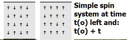
The "Ising model" is central to many problems and systems in statistical mechanics.  It first came to the fore in the study of ferromagnetic systems. It was found that the use of such simplified models paved the way for greater understanding via modeling of more complex systems.  Let's now look at an elementary, statistical mechanical spin system.  A fairly  mundane example is a two-dimensional Ising model for ferromagnetic matter. It contains magnetic domains for which the individual spin magnets can be subject to sudden reversals. For a simple example, think of the 2D model of 4 x 4 elementary spin magnets as shown below:

 
Here the Ising model system, by virtue of undergoing spontaneous magnetization  discloses an evolution to a higher degree of order  (from state S(1) to state S(2)) at the later time t(0) + t, where t could be in billions of years or nanoseconds.

The degree of order, as well as information, is determined from what is called "the spin excess", or the net spin difference (up minus down or vice versa). The larger this number, the greater the degree of order, and the lower the entropy of the system. Obviously, since 0 denotes an extremely low number, we can deduce large entropy.

Consider the system S(2) in more detail, noting the right side orientations of the elementary spin magnets. Here we get: 14 spin ups - 2 spin downs = 12 spin ups, or in other words the spin excess = 12. This system, S(2), has much higher degree of order (less entropy) than the system S(1). (We should add here that higher entropy - as in S(1) - corresponds to the most probable state, defined by the minimal spin excess of zero.)

Accessing such simple systems allows us to infer fundamental measures applicable to the systems, for example the "magnetic moment" of a state, as well as the "degeneracy function". Consider an N= 2 model system with either 2 ups (two up arrows) or 2 downs. 

Then, if  m  denotes the magnetic permeability we can have:

M = + 2 m   or M = -2 m

where the first is the magnetic moment for two spin- up particles, and the second for two spins down. One can also, of course, have the mixed state inclusive of one spin up plus one spin down, then:

M = O m or O

Meantime, the degeneracy function computes the number of states having the same value of m (individual spins) or M such that:

g(N,m) = N!/ (½N + m)! (½N - m)! [M_av]


where [M_av] denotes the average value of the total magnetic moment summed over all states (e.g. with m_s)

The power of the Ising model, however, doesn't end with ferromagnetic systems. We can also use it to examine ice crystal configurations as has been shown in a recent paper by Andrei Okounkov (Bulletin of the American Mathematical Society, Vol. 53, No. 2, p. 187).  In this paper the author presents us with the 2D ice crystal Ising model shown below:


Each white square denotes an ice crystal and the blue areas represent separating media. Certain model stipulations apply as given in the paper: 1) the total number of white squares is fixed, just as the total number of elementary magnets in the earlier system; 2) all squares along the boundary are deemed blue in order to prevent crystals sticking to the sides of the container, and 3) It must be possible to assign probabilities to the configuration in the same way we might assign "order" or entropy to the ferromagnetic system.

The most basic probability for any such system is "thermal equilibrium". Thus, at some temperature T if the system attains thermal equilibrium then the probability of any particular configuration decays exponentially with the energy of C, which is analogous to E  =  m _m  B in the ferromagnetic case. The probability of any particular configuration dependent on T is then:

Prob (C) = 1/ Z(T) [exp (-Energy (C)/ kT)

Where k is Boltzmann's constant, 1.38 x 10 ^-23  J /K.

One will also make use of the  "partition function":

Z(T) =  å _C   exp (- Energy (C)/ kT)

which as Okounkov notes, really functions as a "normalization factor"  given that it "makes the probabilities sum to 1".  In this Ising ice crystal model, then, the energy is "the sum of interactions of all adjacent squares." Since the total number of squares is fixed (see stipulation (1))  then the energy must be proportional to the total length of the contours separating white from blue.

To identify the contours is easy. If the energetic reader will run off  a copy of  the image of the 2D rectangle, then take a black magic marker and trace around each ice crystal region as it appears, he will have generated the contours. The normalization for energy is then (op. cit.):

Energy = 2 x Length of contours

As in the case of the ferromagnetic system entropy competes with order (energy).  In the Ising ice crystal energy is saved via clumping. If we designate an "order parameter" such that  b = (kT)^-1  then in the ice crystal case the larger   b   the stronger tendency for order. Interestingly, as Okounkov notes there is a critical temperature  T_c  > 0 above which entropy wins, it is:

b  =  0.5 ln ( Ö 2    + 1)  

Below T_c  and for ice crystal concentrations above a certain threshold a crystal will form as the size of the container goes to infinity.

Problems:

1) Quantify the magnetic energy for the system at time t(o) compared to time t(o) + t, if the magnetic energy of one spin magnet can be written:

M = - m B cos Θ

where m  is the magnetic moment (-eL/2m, L = 1) and assume Θ = +/- π, and B = 0.1T. 

2)  Say that S = log (g) determines the entropy for a  simple statistical mechanical system, where g denotes the number of accessible states. Then estimate S for the 2D ice crystal model - including any errors that might enter.

Looking At Simple 2D Ising Models

The "Ising model" first came to the fore in the study of ferromagnetic systems. It was found that the use of such simplified models paved the way for greater understanding via modeling of more complex systems.  A fairly  mundane example is a two-dimensional Ising model for ferromagnetic matter. It contains magnetic domains for which the individual spin magnets can be subject to sudden reversals. For a simple example, think of the 2D model of 4 x 4 elementary spin magnets as shown below:



 Here the Ising model system, by virtue of undergoing spontaneous magnetization (say from a state S(1) with spin excess 0 to state S(2) with spin excess 12 , discloses an evolution to a higher degree of order at the later time t(0) + t, where t could be in billions of years or nanoseconds.

The elementary magnets may exist temporarily in the state S(1) as shown  (i.e. each arrow denotes the net spin of the atom based on the sum of electron orientations within it). We then may want to find the degree of order applicable to the system, say at time t(o) and do the appropriate counting of "spin ups" and spin downs" as shown in the left side of the model.  We find on doing so (which the reader can verify) that we get 8 spin ups - 8 spin downs = 0 net spin, or in other words the system is at equilibrium.

Consider then the same system but at a later time (t(0) + t) , for which we behold the right side orientations of the elementary spin magnets. Here we get: 14 spin ups - 2 spin downs = 12 spin ups, or in other words the spin excess = 12. This system, call it S(2), has much higher degree of order (less entropy) than the system S(1). (We should add here that higher entropy - as in S(1) - corresponds to the most probable state, defined by the minimal spin excess of zero

The degree of order, as well as information, for the simple spin system shown is determined from what is called "the spin excess", or the net spin difference (up minus down or vice versa). The larger this number, the greater the degree of order, and the lower the entropy of the system. Obviously, since 0 denotes an extremely low number, we can deduce large entropy.

Accessing such simple systems allows us to infer fundamental measures applicable to the systems, for example the "magnetic moment" of a state, as well as the "degeneracy function". Consider an N= 2 model system with either 2 ups (two up arrows) or 2 downs. Then, if m denotes the magnetic permeability we can have:

M = +2m or M = -2m

where the first is the magnetic moment for two spins up particles, and the second for two spins down. One can also, of course, have the mixed state inclusive of one spin up plus one spin down, then:

M = O m or O

Meantime, the degeneracy function computes the number of states having the same value of m (individual spins) or M such that:

g(N,m) = N!/ (½N + m)! (½N - m)! [M_av]


where [M_av] denotes the average value of the total magnetic moment summed over all states (e.g. with m_s)

The power of the Ising model, however, doesn't end with ferromagnetic systems. We can also use it to examine ice crystal configurations as has been shown in a recent paper by Andrei Okounkov (Bulletin of the American Mathematical Society, Vol. 53, No. 2, p. 187).  In this paper the author presents us with the 2D ice crystal Ising model shown below:

Each white square denotes an ice crystal and the blue areas represent separating media. Certain model stipulations apply as given in the paper: 1) the total number of white squares is fixed, just as the total number of elementary magnets in the earlier system; 2) all squares along the boundary are deemed blue in order to prevent crystals sticking to the sides of the container, and 3) It must be possible to assign probabilities to the configuration in the same way we might assign "order" or entropy to the ferromagnetic system.

The most basic probability for any such system is "thermal equilibrium". Thus, at some temperature T if the system attains thermal equilibrium then the probability of any particular configuration decays exponentially with the energy of C, which is analogous to E  = m _m  B in the ferromagnetic case. The probability of any particular configuration dependent on T is then:


Prob (C) = 1/ Z(T) [exp (-Energy (C)/ kT)

Where k is Boltzmann's constant, 1.38 x 10 ^-23  J/K.

One will also make use of the  "partition function":

Z(T) =  å _C   exp (- Energy (C)/ kT)

which as Okounkov notes, really functions as a "normalization factor"  given that it "makes the probabilities sum to 1".  In this Ising ice crystal model, then, the energy is "the sum of interactions of all adjacent squares." Since the total number of squares is fixed (see stipulation (1))  then the energy must be proportional to the total length of the contours separating white from blue.

To identify the contours is easy. If the energetic reader will run off  a copy of  the image of the 2D rectangle, then take a black magic marker and trace around each ice crystal region as it appears, he will have generated the contours. The normalization for energy is then (op. cit.):

Energy = 2 x Length of contours

As in the case of the ferromagnetic system entropy competes with order (energy).  In the Ising ice crystal energy is saved via clumping. If we designate an "order parameter" such that  b = (kT)^-1  then in the ice crystal case the larger b   the stronger tendency for order. Interestingly, as Okounkov notes there is a critical temperature  T_c  > 0 above which entropy wins, it is:

b =  0.5 ln (Ö2    + 1) 

Below T_c  and for ice crystal concentrations above a certain threshold a crystal will form as the size of the container goes to infinity.

From this brief foray iwe can see that  the Ising model shows the great generality of physics, in being applicable to vastly dissimilar physical entities.

Looking At Stellar Emission and Absorption Processes (1)

In a previous set of blog posts from three years ago, e.g.

http://brane-space.blogspot.com/2012/04/simple-solar-radiative-transfer-1.html

I examined the basic conditions for radiative transfer in a stellar medium or atmosphere. Of course, this is barely one half the story. Ultimately, the solar physicist examines radiative transfer to obtain first clues in how to understand emission and absorption processes which can occur in that atmosphere.

In this post we examine details of emission and absorption in terms of what are called transition probabilities.  Basically one can consider and evaluate three possible cases:

i)                   A stimulated emission probability

ii)                 A spontaneous emission probability

iii)               An absorption (or negative emission) probability

We will use a condensed notation in order to not have too much notation clutter within a limited blog post space To do this we will apply the following symbols to the differing probabilities:

A₂₁ = spontaneous emission probability;  I _{u 21} B ₂₁  =  stimulated emission probability,  and lastly,   I _{u 21} B _12.   =  absorption probability 

    Of critical importance in considering transitions between energy states are the statistical weights of the states, which we denote by g. Then given statistical weights[1], say g₁ and

g ₂, we first wish to show that:

g₁    B _12.  =   g ₂ B ₂₁

 In other words, the absorption probability for state g₁ must be equal to the stimulated emission probability for state g_2..  There can’t be more transitions than the numbers of electrons available for them in those states. For thermal equilibrium, especially, we have detailed balancing. i.e. the number of transitions from level one to level two must be equal to the number of transitions from level two to level one.

From level 1 to level 2 we may write:  N₁ I _u  B _12.

From level 2 to level 1 we write:  N₂  (A₂₁   +  I _u  B _12.)

For detailed balancing we require:

 N₁ I _u  B _12.   =  N₂  (A₂₁   +  I _u  B _12.)

We note here that in thermodynamic equilibrium Boltzmann’s equation applies:

N₂ / N₁   =  I _u  B _12./ (A₂₁   +  I _u  B _12.) =  

 [g₂ / g₁ ]   exp (- E2 – E1) / kT

Where E2, E1 designate the respective energy levels.

Then:  I _u  =  2h u ³ / c ²  [1/ exp (hc/lkT]

As T ® ¥     and  I _u  ® ¥  

 Then:

  B _12./ B ₂₁    =  g₂ / g₁   or   g₁    B _12.  =   g ₂ B ₂

We also need to show, for detailed balancing:

A _21./ B ₁₂    =  2h u ³ / c ²  [g₂ / g₁ ]

We use:

I _u  B _12. =  

(A₂₁   +  I _u  B _21.) [g₂ / g₁ ]   exp (- E2 – E1) / kT

And:

I _u [B _12.- B _21. (g₂ / g₁ )  exp (- E2 – E1) / kT]

 =    (A₂₁)  (g₂ / g₁ )  exp (- E2 – E1) / kT

®  I _u [B _12.- _. (g₂ / g₁ )( g₁ / g₂) B ₁₂  exp (- E2 – E1) / kT

I _u =  A _21./ B ₁₂  (g₂) e ^{(- E2 – E1) / kT}/ g₁  [1 - e ^{(- E2 – E1) / kT}]

=       A _21./ B ₁₂  (g₂ / g₁ ) [e ^{(E2 – E1) / kT}   -   1]

=   2h u ³ / c ²  [1  / e ^{hu / kT}   -   1 ]

And:   

A _21./ B ₁₂  (g₂ / g₁ ) =    2h u ³ / c ² 

Then:   A _21./ B ₁₂    =  2h u ³ / c ²  [g₂ / g₁ ]

Thus, we see that in thermodynamic equilibrium, the ratio of populations in upper and lower levels is given by the Boltzmann formula. In most solar applications of interest, the stimulated emission is negligible compared to the spontaneous emission.

     Note also that Einstein showed that the transition probabilities are related by:

A _21.=  8 p h u ³ / c ²  [B ₂₁] =  8 p h u ³ / c ²  (g₁ / g₂ ) B ₁₂    = 

6.67 x 10 ¹⁶ [g f/g2  l²   Å]

Where g is the Gaunt factor, of order unity and f is the oscillator strength. The latter generally has specific values for discrete transitions. (For the strongest spectral line from a level one in an atom one can usually use f = 1.

The radiation density is defined:

u _u =  4 p  B _u /  c  =  8 p h u ³ / c ²  [1  / e ^{hu / kT}   -   1]

With the Planck function:

B _u  du   =  2h u ³ / c ²  [1  / e ^{hu / kT}   -   1 ] du

This is for the frequency domain, but can also be expressed in the wavelength domain:

B _l  dl   =  2 p h c ² /l⁵   [1  / e ^{hc / kl T}   -   1 ] dl

(Be careful treating the differential for  the frequency!)

du  = (- c/ l²) dl which must be used when transferring from the frequency scale Hz ^-1 to the wavelength scale

 (cm ^-1 or m^-1)

For hydrogenic atoms (Z » 1) the absorption cross-section, a _u , plays  a critical role, defined:

a _u  = 2.815 x 10 ²⁹    Z ⁴/ n ⁵ (g /u ³)

Or:

a _u  =  7.91 x 10 ¹⁶   Z ⁴/ n ⁵  (R_y / h u)³  g

(cm ² / bound electron in state n.)

Where R_y  is the modified Rydberg constant for atomic physics.  In terms of the standard Rydberg constant, R_∞ = 1.0974 × 10⁷ m⁻¹, it is:   R_y  = hc R_∞  = 13.605 eV.

When dealing with complex atoms one needs to allow for the number of electrons in the absorbing state:

a _u  =   4 p/ c  (B _ne) h u

where B _ne is the Einstein coefficient or “continuum f-value”. Thus, it may also be posed:

a _u  =  8.067 × 10^-18      (df/de) 

(cm ² / bound electron in state n.)

A useful table that will come in handy for spectral line computations is the following:

Quantum Numbers and Energies For Hydrogen Atom:

Ground state s1       n    ℓ     m ℓ       m s	Energy E1 (eV)
1     0      0        +½ 1     0      0        -½	-          - 13.6 -         - 13.6
First Excited States n    ℓ     m ℓ       m s	Energy E1 (eV)
2     0       0       +½	-          3.40
2     0       0       -½	-          3.40
2      1      1      +½	-          3.40
2      1      1       -½	-          3.40
2      1      0      +½	-          3.40
2      1      0       -½	-          3.40
2      1      1      +½	-          3.40
2       1      1      -½	-          3.40

Inspection of the table above shows two quantum states with the same energy (-13.6 eV) and eight states with (-3.40 eV).  Thus, two states are degenerate for the n=1 level and eight states are degenerate for the n=2 level.  Since g _n = 2n², then:

At the n=1 level the statistical weight is:  g ₁ = 2(1)² = 2

At the n=2 level the statistical weight is: g ₁ = 2(2)² = 8

Problems for Budding Astrophysicists:

1)Consider a gas of neutral hydrogen. Using the Boltzmann equation and the information in the table above, compute the temperature at which one will expect equal numbers of atoms in the ground state and the first excited state.

2) For the Balmer a line (called H- alpha), we know:

E3 – E2 =  - 13.6 eV ( 1/ 3 ²   -  1/ 2 ² )   = 1.88 eV

a)     From this information calculate the ratio N₂ / N₁    for T = 10 ⁴ K

b)     Obtain the specific intensity from: 

I _u  =  2h u ³ / c ²  [1/ exp (hc/lkT]

3)Calculate  the transition probability (  A ₂₁  ) you get using the Einstein equation:

 If:   A _21.=     6.67 x 10 ¹⁶ [g f/g2  l²   Å]

What possible errors might cause the values to diverge? (Take g = f » 1)

---

[1] The “statistical weight” or degeneracy is just the number of different atomic sub-states included in the state being considered.  As we saw each atomic state of angular momenta L,S leading to total angular momentum J can be split by magnetic field into 2J + 1 states. Then for all J levels of a term LS there are: 

g(L.S) = (2L + 1)(2S + 1) = S _j (2J + 1)

different M _j sub-levels possible. For a hydrogenic shell (n) there are  2n ²  sub-levels possible.