The Parker Solar Probe - Why It's A Monumental Engineering Feat - And The First Image Delivered

Artist's conception of the Parker Solar Probe which will approach within 4 million miles of the Sun.   

The level and rate of successes - including newly processed imagery- of the latest solar space craft are almost too numerous to tally. One can then understand-  even if one is not a solar physicist - why the Parker solar probe had been renamed from the original "Solar Probe Plus".   In this post I want to examine why the Parker solar probe has been such a success, especially in terms of the engineering components and the associated experiments to be carried out over its 7-year mission. (Okay, actually 6 years and 321 days)

In terms of solar physics there is perhaps no more towering personage than Eugene Parker. Indeed, it was reading his original research papers on the magnetic structure of sunspots - portrayed as assemblies of multiple flux tubes - that enticed me to go into the field of solar physics 40 years ago.

Why is Eugene Parker so special ?  Well, to many of us who've invested segments of our lives into solar research he is seen as the father of solar physics. It was while Dr. Parker was still a budding young astrophysicist at the University of Chicago that he wrote a seminal paper in 1958 about the solar wind and its association with the interplanetary magnetic field. (Parker, E.N. : Dynamics of the interplanetary gas and magnetic fields,” 128, 664, Astrophys. J., 1958.) The paper can be accessed at the link below for those interested:

http://adsabs.harvard.edu/full/1958ApJ...128..664P

Fast forward some 21 years, to ca. 1979. Measurements over decades of the so -called Evershed effect showed the plasma motions to be radial and inwards. There did not appear to be any 'escape hatch' for the rising gas columns represented by the umbral dots. This being the case sunspots ought to heat up and reach equilibrium with the surrounding photosphere after a few days, and yet spots with umbral dots were observed to last weeks.

And so the "multiple flux tube" model of Eugene Parker was born (cf. Astrophys. J., 230, 905-13). In the diagram shown below note the geometry of the field lines extending from beneath the photosphere (in the convective zone) to far above it. The 'flaring field' on top is buoyant for reasons that have to do with the stratification of the solar atmosphere. The Wilson depression is shown as the indentations at the umbral surface on either side.

Parker in his paper (ibid.) showed that the downdraft velocity needed to remove heat from beneath a sunspot  (at a depth of 2500- 5000 km) is on the order of the Alfven velocity  e.g.

v  _A   = B_o  / [m _o  r _o]  ^{1/ 2}

for this region, where   B_o  is the equilibrium magnetic field, m _o   is the magnetic permeability of free space,  and r _o   is the plasma density. This leads to v  _A   =  about 2 kilometers per second. This then is adequate to provide the observed umbral energy flux of 0.2 F _o  where F _o  denotes the normal photospheric flux.

The full paper can be accessed here:
http://articles.adsabs.harvard.edu//full/1979ApJ...230..905P/0000905.000.html

A key fact relevant here is that heat flux and magnetic field strength is independent of sunspot area. The parameter that best helps to explain this is the vertical distance 'x'  which the model predicts is characteristic of all sunspots whether they be 4,000 km or 40,000 km across. Calculations by Parker show x = 1150 km approximately. It is the limiting distance below which an instability would occur in a single flux tube.

From all these points of view, the adoption of Eugene Parker's name for this one of a kind  solar craft - the first ever long term mission to our nearest star- is welcome and quite understandable. Indeed, the mission is a culmination of Prof. Parker's research in the fields of solar physics and heliophysics (the latter distinguished from the former on the basis of the extent of the solar wind, e.g. into the heliosphere - or the magnetically affected region that extends beyond Pluto's orbit).

Now what makes this solar mission so extraordinary?  First, back in November last year the craft made the first of 24 "oscillating" sweeps into the solar atmosphere. By that I mean the flight path carried it in then back out. In the November approach it came to within 15 million miles of the Sun's surface or photosphere. This is far closer than any earlier craft has ever gone. The previous record was set by Helios B in 1976 and broken by Parker on Oct. 29 — and this maneuver has exposed the spacecraft to intense heat and solar radiation in a complex solar wind environment. 

 Second, Parker features marvelous engineering designs which enable it to make such close passes.  (And bear in mind this was the first of 24 such oscillating in and out orbits, where the sunlit sie can reach as high as 1370 C.)   The main component here is a 2.5 meter wide, 72.5 kilogram heat shield, made of carbon foam sandwiched between two carbon sheets.  The whole shield is only 11. 5 centimeters thick (about 4. 6 inches).  It's coated on the Sun facing side with white ceramic paint to reflect as much sunlight as possible. Even then that side is expected  heat up to more than 1300 degrees Celsius.   Behind it, the bulk of the craft will coll to just 30 C on average, or about 86 F - about like a balmy spring day in Barbados.  

Other features of the Parker solar craft worth noting:

1) A component experiment for 'Integrated Science Investigation of the Sun' which is designed to detect solar particles across a wide range of energies.  This will allow solar physicists to decipher how the Sun accelerates the solar wind.  One detector will search for low energy particles, while a different one will search for high energy ones.  

  2) A component designated WISPR (Wide -field Imager for Solar Probe) will take images of the solar corona, solar wind, shocks and solar flares.  These images will help scientists properly interpret data from the other instruments.   

3) The craft features two solar panels mounted on a movable joint to control how much sun light (radiant energy) the panels absorb.  In close passes to the Sun - such as last November-  the panels will fold behind the heat shield, leaving only a last row of solar cells to absorb energy.   

4)The craft will be able to expel heat through a set of radiators composed of black material, which will be worn like a collar between the heat shield and the bulk of the space craft. Tubes of water will carry heat from the solar panels to the radiators where the heat can then escape into space.  At all temperatures the probe's solar panels will need to stay cool and the design of this system ensures it - especially the fact the panels are threaded with 'veins' to carry cooling water. 

4) Another experimental component, designated FIELDS, is comprised of five antennas to measure electric and magnetic field strengths in the solar neighborhood.  These measurements ought to help us to understand what makes the solar corona so hot (at nearly 2 million K).  To this end, four of the antennas are made of special material to protect them from direct sunlight..  

5) At the back of the probe will be the SWEAP experiment, for "Solar Wind Electrons Alphas and Protons".   This is designed to catch charged particles including electrons, and alpha particles ("alphas") from the solar wind and also determine their temperature, density and speed.  It will be exposed to sunlight 475 times as intense as felt on Earth.  

We can expect much data as well as imagery to be forthcoming in the coming months and years, as this monumental exploration of our Sun proceeds. Already, Parker has captured the image below of the Sun's corona, taken on December 8th.

The Parker solar adventure is just beginning, stay tuned!


See also:

Parker Solar Probe Heat-Resistant Technology - Spacecraft ...

Selected Questions- Answers From All Experts Astronomy Forum (Yellow stars and heated 'yellow' bars)

Question -

I think a yellowish star would have a different temperature from a yellowish heated bar. Could you explain in detail the  difference?

Answer:


The problem in the question, is that you have not referenced WHICH part of
the star you're comparing to the heated bar.

A star, like an onion, has different layers at different temperatures. The
inner core (e.g. for a yellow star like the Sun) is at temperatures of millions
of degrees.

Such high temperatures are attained by virtue of nuclear reactions in the
star's core. The radiation, energy produced then flows outward to the
surface.

The surface (or photosphere) of the star is therefore much cooler, at
temperatures around 11,000 F (for the Sun, a typical yellow dwarf star).

Assuming that you are talking about the surface of the yellow star, the
difference is clearly that the yellow bar could not attain the same
temperature, before melting. The melting point of steel, for example, is
at 2500F.

A star's surface- at the SAME temperature- would result in a red star, not
yellow.

How can this be explained?

Basically, it's a result of the fact that star and metal (bar) are
composed of two different types of materials.

The metal bar is a solid. (E.g. made of steel, or iron) As it is heated,
its electrons become agitated and move around, vibrate - however, they are
limited in where they can go. (Up until the metal melts).

The star, by contrast, is in a state called plasma. This is a gas that has
lost one or more electrons. Once this state emerges, the star can continue
gaining temperature way past the maximum allowed for the solid, metal bar.
(Helped by the fact its ions (atoms that've lost electrons) are not
constrained in their motions).

At the same time, the loss of electrons by a plasma means its electrical
conductivity increases. It can also form magnetic fields, because of its
ability to conduct electric currents.  These currents - as well as the
associated magnetic energy - can also convert into more heat energy- and
also power flares.

All these aspects help explain why a yellow star is fundamentally
different from a heated yellow bar. (For example, no matter how much you
heat the bar- short of its melting point- it won't produce magnetic fields
like moving fluid in a heated plasma will!)

Bottom line is that the plasma nature of the star allows more heat to be
absorbed by it, and brought to its surface, than the atoms of a heated bar
allow.

Lastly, one needs to bear in mind that the yellow bar radiates at that
particular energy range alone. The yellow star radiates at all wavelengths
of the EM (electromagnetic) spectrum, including x-rays, UV rays, radio
waves  and so on.

But it radiates its peak (of what is called the 'black body curve' or
Planck curve) in the yellow region of the visible light spectrum. In
effect, stars of whatever color actually radiate at all wavelengths but
at different intensities for each. It is the peak of the radiated energy
that defines the color of the star we see.

What Aspects Of The Coming Total Solar Eclipse Are Most Critical For Astrophysics?

Image showing totality in a previous  solar eclipse. The Sun is totally blocked out by the Moon - in the line of sight- and the solar corona is seen expanding from the solar limb


Graphic showing the path for Aug. 21 total eclipse - and the partial zones to either side, with the percentages of the Sun to be covered.

As we approach August 21 and the first total eclipse to appear in in the U.S. in38 years, many are trying to stay ahead of the fervid hype. Here are the only two things you need to know: 1) In most of the U.S. the eclipse will be seen as partial only and you need special glasses in order to observe the transition to maximum coverup, and 2) If you want to observe the total eclipse (see top image) you will have to travel to some place within the band of totality (see graphic).  For example, in our location (Colorado Springs) the Sun will be roughly 85 percent covered.

Here's the skinny on stats for this eclipse: Approximately 12 million Americans will be directly in the totality band shown in the graphic. Another 88 million will be within 200 miles of some place inside the totality band. Naturally then, those living in communities right in the band (e.g. Jackson Hole, WY, St. Joseph, MO) are expecting eclipse watchers to pour in and pump up their economies - buying t-shirts, special glasses and other paraphernalia.

While the basic image of totality will be the appeal for casual observers,  and even partial eclipse will occur for (and excite)  many others, this doesn't hold quite the same spell for solar physicists or astrophysicists. They look to good observations made during totality, namely to be able to record and analyze the solar corona.   This is the outermost region of the solar atmosphere, at millions of kelvins temperature and extending sometimes millions of kilometers into space.

The corona up to now has presented a mystery, especially in terms of its "inverse" increasing temperature profile considered in the context the general temperature profile is steadily decreasing from the Sun's interior to outside.   For example, the Sun's "surface" or photosphere has an effective temperature of 5,777 K .   The corona's temperature by contrast is at least 2 million degrees K.

How did we find this out?  The key breakthrough probably arrived in 1939 when astronomer Walter Grotrian found that a previously discovered spectral line (attributed to "coronium") was actually 13 times ionized iron. Since it takes enormous energy to ionize even one iron atom (meaning stripping one of its outer electrons away) this meant the iron had to be subject to enormously high temperatures.  Indeed, such ions can only exist in plasmas with temperatures between 1 million and 5 million K.

The first clue as the cause of the extraordinary hearing came with high altitude rocket flights in the 1970s, bearing x-ray telescopes. These showed  features down to a resolution of 1 arcsec or 730 km.  Careful observations showed a positive correlation between the x-ray brightness of active regions (i.e. containing complex sunspots) and plasma-filled magnetic loops, e.g.



















The above image was taken by the much more recent Atmospheric Imaging Assembly, built for the Solar Dynamics Observatory . But you easily get the idea noting the brightness (representative image taken at  211Å) and the magnetic loop structures.

Another milestone occurred when Eugene Parker predicted the hot corona must expand into space as a solar "wind". It could not remain stationary or in place with no expansion. The proof of this is left at the end for those interested.

The next question, of course, is where the energy comes from not only to heat the corona but accelerate the solar wind which is an extension of it.  We believe now that MHD or "magnetohydrodynamic" waves of some type provide an answer.   Field lines such as shown in the previous image are rooted at both ends in the Sun's convection zone where they are jostled by the churning of convective cells.  If sufficiently rapid these field line motions could generate magnetic waves capable of carrying energy upward into the loop.   It seems that Alfven waves e.g.

http://brane-space.blogspot.com/2011/04/getting-handle-on-alfven-waves-2.html

are the most effective in reaching coronal heights. (Alas, Alfven waves do not compress the ambient plasma so we still need to identify some other mechanism that can effectively transfer the wave energy to the plasma. A clue may lie with Landau damping, say associated with a beam (or 2-stream)  instability in the plasma. We have a dual Maxwellian profile.


In the region where the slope is positive (¶f(v)  / ¶ v > 0) there is a greater number of faster than slower particles so a greater amount of energy is transferred from particles to associated (e.g. Alfven) waves.  Since f _eb contains more fast than slow particles a wave is excited.

But in Landau damping, with the slope negative (¶f(v)  / ¶ v < 0) the number of particles slower than the waves phase velocity exceeds the number of those that are faster. Thus, more particles gain energy from the wave than lose energy to it.

Whatever new data the eclipse generates, and there will be lots of it, we can be confident that the mysteries of the solar corona won't be solved even after it's all analyzed and multiple papers published. But I will keep readers abreast of any new findings say that appear in the next 8-12 months.

Those interested in actual scientific participation are invited to go to the Globe Observer site, where you can collect the app and then be prepared to make temperature measurements.

https://observer.globe.gov/

See also:

https://www2.mps.mpg.de/meetings/ccmag/dokumente/presentations/A.04.06.pdf

----------
Proof that the corona can't be stationary:

A static corona  superficially appears  to be quite reasonable but that’s why we need to test this is so. The first one to do this was Sydney Chapman. He began by first assuming the condition for hydrostatic equilibrium applied:

dp/ dr = - r {GM_s/ r²}

where G is the usual Newtonian gravitational constant, and r defines the plasma density for the corona, while M_s is the mass of the Sun, and r the distance from the solar center:

r = n(m_p)

with n the number density for protons

The coronal pressure (P) is given by:

P = 2 n T

Provided both protons and electrons are assumed to have the same temperature.

The thermal conductivity of the corona is dominated by electron thermal conductivity and takes the form:

k = k_o T ^5/2

for typical coronal conditions the value of k is about 20 times the value of copper at room temperature.

The coronal heat flux density is:

q = -k Ñ T

A static corona means heat inputs cancel heat outputs so that the divergence:

Ñ× q = 0

Assuming a spherical symmetry for the corona one can write:

1/r² [d/dr (r² k_o T ^5/2  dT/dr)] = 0

    Obviously the preceding assumptions mean there must be some distance where the coronal temperature becomes zero.

From the above equation one should be able to show:

d(T ^7/2) = 7/2 (F T_o ^5/2)/ 4 p k_o d(1/r) = C d(1/r)

where C is a constant.

The integral is:

T_o ^7/2 - T ^7/2 = C[ 1/R_o - 1/r]

Now, set the temperature at infinity (T) to zero and obtain:

C = R_o T_o ^7/2 

which fixes the total flux at:

F = 2/7   [4 p R_o k_o T_o ]

After another step, one finds:

T(r) = T_o (R_o / r) ^2/7

    This gives the temperature T at a distance from the Sun= r. This is based on using a defined value (say T_o = 2 x 10⁶ K) at a defined distance, say R_o = 7 x 10⁸ m.

    For example, at the Earth’s distance (r = 1.5 x 10¹¹ m) one would find: T = 4.3 x 10⁵ K

    This seems fine, until one examines the pressure.

    Analogous to the temperature formalism, we have, the pressure p(r) at some distance r defined by:

p(r) =

p(R_o) exp [7/5 GM_s m_p/ 2 T(R_o) R_o {( R_o / r)^5/7 – 1}]

    Now, if one allows r to approach infinity, e.g. r ®¥ an interesting thing occurs in the equation, as we can see. That is, the denominator of the first term in the end brackets becomes so large (R_o / ¥) that the first term vanishes.

Then we are left with the expression for the pressure:

p(¥) = p(R_o) [exp – 7k/5 * 1/ T(R_o) R_o]

where ‘k’ denotes a constant composed of all the constant quantities in the previous eqn. (G, M, m_p etc)

    Substituting the given values into the above, one finds p(R_o) multiplied by a factor

exp[0] = 1

    The reason is that the exponential of a very small and negative valued magnitude ® 0

Then:

p(¥)  »  p(R_o)

But this can’t be since the pressure of the coronal base would then be the same as the value at infinity!

    This led astrophysicists to conclude an unphysical result, and that the static coronal model couldn’t be accurate.

    If the static model were accurate, the pressure at infinity should be zero, p(¥)   = 0, not a small finite pressure that’s effectively equal to the coronal base pressure. This finding led to the further investigations that disclosed a solar “wind” had to flow outwards from the corona.

New Space Weather Model Enhances Solar Wind Insights

Space weather, entailing the useful forecasting of major events such as solar flares and coronal mass ejections (CMEs),  isn't merely of academic or abstract interest. This is because we know major adverse events can knock out our satellites, as well as disrupt telecommunications systems, not to mention affect the navigational instruments on aircraft.

For years, ever since the mammoth project I described some time ago, based on this released monograph:

http://brane-space.blogspot.com/2015/04/one-of-most-massive-scientific-projects.html

we've also known that forecasting serious events  requires a solid understanding of the solar wind, a 1, 610,000 kph stream of charged particles constantly emitted by the Sun in all directions. However, solar wind dynamics are maddeningly complex as the original contributors to the Solar-Terrestrial Predictions Workshop held in Meudon, France learned.

Now, new research by Feng et al (Journal of Geophysical Research, Space Physics, 2015) discloses a different approach and also improves on previous efforts to model the solar wind.  This model is driven by real world data, from which it predicts the behavior of the solar wind from the moment it leaves the Sun until its arrival at Earth.

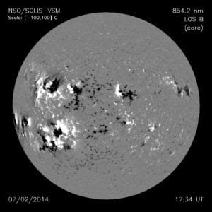
Feng's team based this new model on an older magnetohydrodynamic simulation that predicts the behavior of an electrically conducting fluid (the solar wind in this case) in the presence of a magnetic field. This older model relies on daily maps of the Sun's light emitting layer known as the photosphere. Such an image, from a vector magnetograph, is shown below:


In the image shown above, for example, the (+) magnetic polarities are visible as bright regions, contrasting with the (-) polarities in dark.   To improve the older simulation, Feng et al changed the way the daily magnetic field data are processed and used by the model. They also added a limit on the mass flux of the photosphere, that is, the energy it emits over a given surface area.

The team then tested the new model's predictions against solar wind predictions from July 1 to August 11, 2008. The model was found to accurately predict specific features in the corona including dark coronal holes and their corresponding streamer 'belts' (the bright rays seen emanating out during a total solar eclipse).  The model also accurately predicted interplanetary solar wind behavior.

Unfortunately, the model was less accurate at predicting the total magnetic field strength during the observation period. Hence, improvements are needed but the Fong et al model can definitely help to make better predictions about space weather, including extreme events like coronal mass ejections.

At the very least the model enhances forecasting from where it had been and that is a win for solar physics.  The bottom line is that plasma behavior under the influence of powerful magnetic fields is often chaotic, as opposed to deterministic. This is what leads to more 'stochastic' forms of prediction which by their very nature harbor significant uncertainty.

As more data are accessed, from diverse instruments, and refinements made via computer processing and imaging, we may finally be on the way to more confident space weather forecasts.

See also the latest space weather forecasts, etc. at:

www.spaceweather.com