The pair basically developed an explanation for the observed distribution of supermassive black hole masses and luminosities, for which there was previously no scientific explanation. Arpan Das in his presentation began by noting the importance of the work given it provided a basis for the formation and growth of supermassive black holes over cosmic time. In addition, the results provided an insight into the formation and evolution of the first massive galaxies in the universe, as well as a history of cosmic re-ionization.
As Das explained it, the original quandary became how to explain the existence of supermassive black holes of mass approaching 10 9 solar masses, at a pronounced red shift of z ~ 7, when the age of the universe was less than 1 billion years. In other words, "how did this get so big, so massive, in so short a time?"
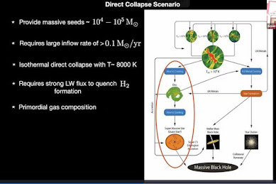
One of the most useful approaches was to invoke the "direct collapse scenario". This was illustrated by Das using the slide shown below:
Here, the content is mostly self-explanatory. Thus instead of having to go through the intermediary stage of forming a massive star, you directly collapse a large molecular cloud into a massive black hole. This provides "seeds" of masses from 10 4 - 10 5 solar masses, which is then "easy to grow into a supermassive black hole of 10 9 solar masses in less than 1 Gyr time". However, as Das pointed out, one also needs secondary conditions to apply, including:
- A large inflow rate (accretion rate) greater than 0.1 solar mass per year
- It has to be an isothermal collapse with T ~ 8,000 K (i.e. no jumps in temperature over the time scale).
- There can be no metals, or hydrogen molecule (e.g. H2) formation which would introduce cooling - so the hydrogen and any metals need to be removed from the gas. Here Lyman-Werner radiation- with photons in the energy range 11.2 - 13. 6 ev is needed to quench H2 formation. (The particular details, which Das did not go into, are found in the previously referenced Ap. J. Letters paper).
The end result of the work then was to "build a mass function but which has to be connected to the primordial history of the black holes" This mass function is given in the following slide:

The use of the initial mass function (IMF) comprised the first step, by which the relevant models were taken from Ferrara et al 2104. This is based on a log (base 10) model, while the growth model is based on an exponential growth rate, i.e.
M(t)/ M o = exp g t
The problem with the number density - differential equation at lower right, is that it's currently unconstrained and not truly empirical so "whatever we have we have to believe in it at the moment" . Fortunately, everything is analytical and you don't really see these at really high density.
The remaining step entails a basic integration, i.e. as shown in their paper, e.g.

Using: f(t') = l exp ( - l t') / [1 - exp ( - l T)]
which results in the final mass function as shown below:

Note here the "erf" or error function - is a mainstay in mathematical physics. Note that all the (Greek- letter ) parameters at the bottom are related to the history of the black hole. E.g. l is the growth rate tied to the direct collapse of a molecular cloud while g defines the growth rate tied to individual seeds in the direct collapse.
After briefly describing these, Das presented the table summarizing the parameters.

He noted that the two top (boxed) parameters arrive from the initial mass function, while the boxed lower parameters are from the growth rate functions derived from the black hole history (referred to time T). Assembling all the above parameter values (obtained from their models for the DCBH growth era) yields a "tapered power law distribution" as shown below:

As noted by Das there is a break (intersection) in the blue and green lines, but none in the red line. The break, notable in the power law at high mass "is really important" as it is a marker for the end of the DCBH growth era. (Since both the creation of new direct collapsed holes and the super -Eddington growth ceases after the time interval T.
Interestingly, these power law parameters can be applied to quasars. Thus, the mass function of high redshift (e.g. high z) quasars can be described by a tapered power law such as shown in the previous slide. The parameters of the power law are determined by the initial mass function and the growth history of the DCBH seeds. The resulting quasar luminosity function is shown below:
The mass function can then be fitted with the observed quasar luminosity function to constrain the growth models of the DCBH. According to Das: "The basic idea was to start with something simple and then make it more complicated like any other model". The beauty of the method is that the equation for the Eddington luminosity, e.g.
LE = 4p c G m p M / s T
Can then be used to transform the mass function into a luminosity function. The final slide then shows the inferred quasar luminosity function: QLF ~ dn / d log L, for a suitable pair of values a , b overlaid on z = 3 quasar (bolometric) luminosities. These were compiled by Hopkins et al (2007) and the fit can be compared by inspection of the preceding graph for the QLF. Effectively, the observations were fit with just the two parameters a , b and the results were not bad at all. Both Basu and Das merit kudos and commendations for their work!


No comments:
Post a Comment